The Loss Function

In order for our neural net to “learn” we first need some measure of how it is doing. This is called the loss function. It measures how far off the output of our net is from what we expect it to be.

There are many kinds of loss function but they all require two values:

1. The real output from your net
2. A label (the output you were expecting)

We will be using a loss function called mean squared error loss. The formula looks like this:

• = the label
• = the output

In English: for each output we subtract the label (expected value) from the output, square that value, then sum all of those squared errors together. We then divide by the number of output/label pairs in the training data times 2.

Here’s the code:

def loss(outputs, labels):
    return sum([(x - y) ** 2 for x, y in zip(outputs, labels)]) / (len(outputs) * 2)

How Do We Reduce the Loss?

It’s useful to think about our neural net not in terms of code, but as a mathematical expression.

We have a loss function which is ultimately the result of a complicated mathematical expression — the inputs of our net being passed through all of the weights and biases of the network, then that final output being evaluated by the loss function.

The weights and biases of the network were just chosen at random. We didn’t know which weights and biases to pick. But what if we could know?

What if we had a number that could tell us how to change the weights and biases of the networks so that we could bring the value of the loss function down to 0? If we did that then our neural net would work perfectly on our training data. We would get exactly the output we were expecting.

If you are familiar with calculus you know that there exists such a number. It is called the derivative. More precisely, it is the partial derivative of the loss function with respect to the weight/bias:

Finding Derivatives

The simplest way to find the derivative of a specific weight in the network is to make some small change to the weight, and observe how that change affected the output of the loss function:

We could do this for each of the weights and biases in the network to find their derivatives.

Gradient Descent

That’s all well and good, but how do we use these derivatives to bring the value of the loss function down? Our goal is to find the global minimum of the loss function.

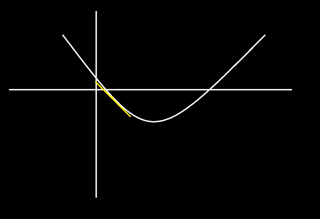
Imagine the graph of a simple function:

Obviously it’s not difficult to find the global minimum of this function analytically. In this case you can tell where it is just by looking at it. This is a function in 2 dimensions — it is very simple. As the function becomes more complicated it becomes prohibitively expensive and difficult to find the global minimum analytically and so we employ an optimization: gradient descent.

The derivative is the slope of the tangent line as you move in the direction of the variable. For example, in the drawing above as we move in the x direction, the slope of the line tangent to the graph changes. The slope is negative and its magnitude gradually decreases until we reach the minimum, where the slope is 0, then it begins to increase.

What we are doing when we iteratively perform gradient descent is:

1. Evaluate the value of our loss function at a certain point (with the parameters we have). In the simple function drawn above this would be plugging in an x value and finding what y value you get out. In our neural net it is computing the forward pass.
2. Find the gradients of the parameters. In this graph example above it is the slope of the tangent line at whatever x value we chose.
3. Move some small step in the opposite direction of that gradient.
4. Repeat.

For instance, say we pick some arbitrary starting x value for our function above and plug it in. Let’s start with . We plug that in and find the slope of the tangent line at that point which might look something like this:

Let’s call that slope . Another way of saying that is:

If we step some small amount in the opposite direction of that gradient, say , our new value would be

Now we evaluate the function again at , and find the new gradient. Let’s call that slope . So our new will be

As we continue this process the magnitude of the gradient decreases and we approach the global minimum of the function.

This function is a very simple function of only 1 parameter. Very complicated neural nets have millions of parameters (sometimes billions), but gradient descent works just the same:

1. Evaluate the loss function
2. Find the gradients of the weights and biases
3. Move each weight and bias in the opposite direction of the gradient
4. Repeat

The “small amount” we choose to move the parameters is called the learning rate. It is often represented with the Greek symbol . This is what’s known as a hyperparameter. It is not a parameter of the neural net itself. It is chosen by us. Different learning rates work better for different functions.

There is an art to choosing the learning rate. If the learning rate is too low, the net will be trained too slowly. If it is too high, you may suffer from “exploding/vanishing” gradient problems and never find the minimum of the loss function.

There is one other hyperparameter involved in gradient descent: the number of epochs. An epoch is simply an iteration of gradient descent. The more iterations of gradient descent you perform during the training process, the lower your loss will be and the longer it will take.

A Better Way of Calculating Gradients:

We have all of the pieces that we need now to train our neural net. There is one issue, however.

When I described how to find the gradients I said that you could simply increase a weight or bias by some small amount, evaluate the new output of the loss function, then use that value to find the gradient:

While this is a perfectly valid way to find the gradients, it’s extremely inefficient and will not scale beyond the most trivial of neural nets. This is because this would require you to evaluate the loss function once for each weight and bias of the network. If our network has 6000 weights and biases (not even a particularly large network) and 1000 training data (not a large set) we would need to compute the loss function 6,000,000 times to perform a single iteration of gradient descent! This is prohibitively slow. We will need a new strategy for finding the gradients.

Happily, there exists a very efficient algorithm for finding these gradients called backpropagation.

Conclusion

In the next blog post I will go over how backpropagation works, and hopefully give you a good intuition of what exactly we are doing when we perform the backward pass.

Here is the code for gradient descent:

def gradient_descent(self, learning_rate, epochs, training_data, training_labels):
    for epoch in range(epochs):
        outputs = []
        for i, input in enumerate(training_data):
            output = self.forward(input)
            outputs.append(output)
            self.backward(output, training_labels[i])
        for layer in self.layers:
            layer.weight_matrix -= (learning_rate / len(training_data) * np.transpose(layer.weight_gradients))
            layer.biases -= (learning_rate / len(training_data)) * layer.bias_gradients

        self.zero_grad()