The Cross-Entropy Loss Function

The loss function is a crucial component to training neural nets. It allows us to get a measure of how well our neural net is doing.

Let’s take a look at the mean squared error loss:

$L = \dfrac{1}{n}\sum_x\lvert\lvert a - y\rvert\rvert^2$

$a$ is the final output from our net
$y$ is our label (the value we were expecting to get)

Even if you are unfamiliar with the mean squared error loss, it should hopefully be plausible to you that this function could measure the difference between how our network is doing, and how we hope it would do.

Now I will introduce a different loss function; the cross-entropy loss:

$L = -\dfrac{1}{n}\sum_x[y \cdot ln(a) + (1 - y)ln(1 - a)]$

Woah! What the…? Where did this come from?

The Problem with Sigmoid Neurons

Let’s take a step back and talk about a fundamental problem with training a neural network of sigmoid neurons.

Here is the graph of the sigmoid function:

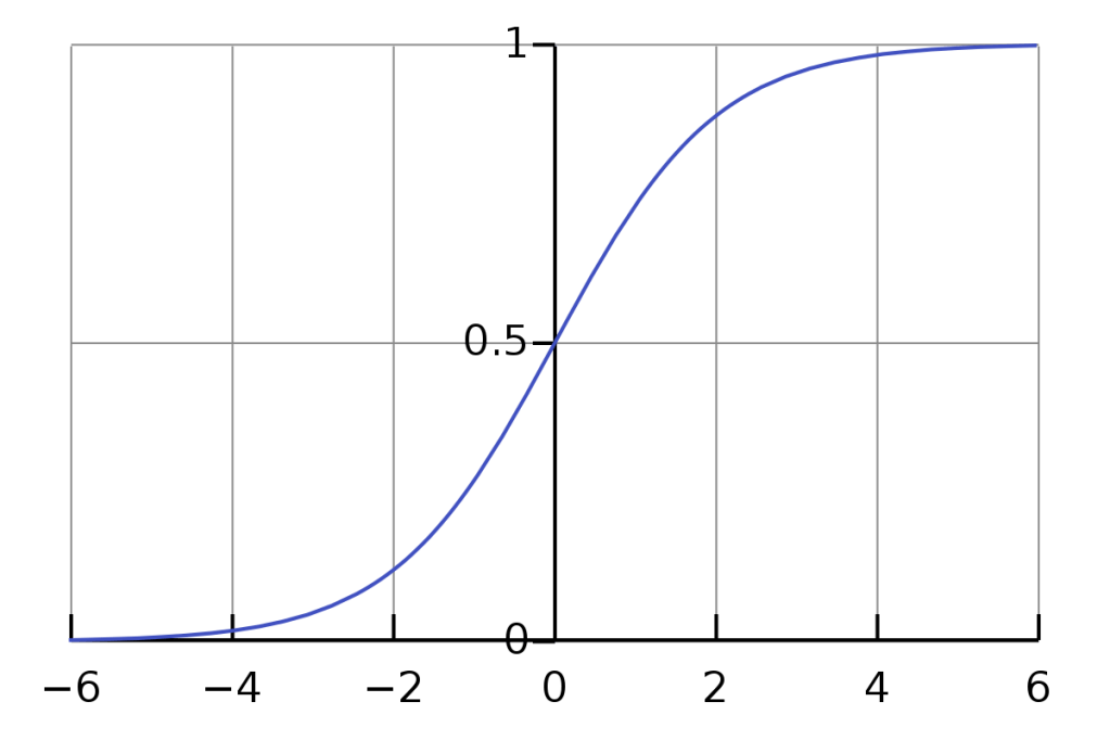
As you can see, the function gets very flat as the inputs to the sigmoid (our weighted sums) get high $(z> 1)$ or low ( $z < 0$ ). In other words, the derivative of the sigmoid function is close to 0 past these points.

This will slow down the rate at which our neural net learns. It is particularly a problem when this 0 term appears in the calculation of the gradients in our output layer, because those gradients will propagate backward into the rest of our net. A tiny gradient in our output layer will slow down learning tremendously.

So what can we do? We want to get rid of the $\sigma'(z)$ term from the gradient equations.

Getting rid of $\sigma'(z)$

The equation for the gradient of the bias is:

$\dfrac{\partial L}{\partial b} = \dfrac{\partial L}{\partial a}\sigma'(z)$

Where $a$ is the final output activation of output neuron. If you recall the equation for the gradient of the bias of an output neuron is (see Understanding Backpropagation):

$\dfrac{\partial L}{\partial b} = a - y \cdot \sigma'(z)$

We want the gradient for the bias to be equal to:

$\dfrac{\partial L}{\partial b} = a - y$

No $\sigma'$ .

We know that the derivative of the sigmoid function is equal to (see The Derivative of the Sigmoid Function):

$\sigma'(z) = \sigma(z) * (1 - \sigma(z))$

In this case, because we are dealing with output neurons, $\sigma(z)$ is just the final activated output of our output layer, $\sigma(z) = a$ . Combining these two pieces of information, we can rewrite the gradient equation as:

$\dfrac{\partial L}{\partial b} = \dfrac{\partial L}{\partial a}a(1 - a)$

Now, let’s plug the value we said we wanted for $\dfrac{\partial L}{\partial b}$ :

$a - y = \dfrac{\partial L}{\partial a}a(1 - a)$

And solve for $\dfrac{\partial L}{\partial a}$ :

$\dfrac{\partial L}{\partial a} = \dfrac{a - y}{a(1 - a)}$

Great! This is the derivative of our ideal loss function. Now, how do we use this to find our ideal loss function? We integrate with respect to $a$ .

Let’s do it step-by-step:

$\int \dfrac{a - y}{a(1 - a)}da$

The first thing we want to do is break this fraction down using partial fraction decomposition:

$\dfrac{A}{a} + \dfrac{B}{1 -a} = \dfrac{a - y}{a(1 - a)}$

To add the two fractions on the left side of this equation we need to get them under a common denominator:

$\dfrac{A(1- a) + B(a)}{a(1 - a)} = \dfrac{a - y}{a(1 - a)}$

Let’s ignore the denominator for now and solve this equation for $A$ and $B$ :

$A(1- a) + B(a) = {a - y}$

We want to plug in values for $a$ that will cause the other term to disappear. To get $B$ to disappear we could set $a = 0$ :

$A(1- 0) + B(0) = {0 - y}$

$A = -y$

Now we want to make $A$ disappear. To do that we could set $a = 1$ :

$A(1- 1) + B(1) = {1 - y}$

$B = 1 - y$

Now we plug those back into our decomposed fraction:

$\dfrac{-y}{a} + \dfrac{1 - y}{1 - a}$

Taking the integral of this will be much easier:

$\int \dfrac{-y}{a} + \dfrac{1 - y}{1 - a}da$

Let’s do it term by term and then combine them together. We’ll start with the first term:

$\int \dfrac{-y}{a}da$

Rewriting it as:

$\int -y * \dfrac{1}{a}da$

Makes it obvious that the integral of this is:

$-y*ln(a) + C$

Now the next term:

$\int \dfrac{1 - y}{1 - a}da$

Once again we will rewrite it like we did the first term:

$\int 1 -y * \dfrac{1}{1 - a}da$

This one is a little trickier, but we will use u-substitution to integrate: Let $u = a - 1$

$\int 1 -y * \dfrac{1}{u}du$

This gives us:

$1 - y * ln(u) + C$

Plugging the substituted value back in:

$1 - y * ln(1 - a) + C$

Now we combine our integrated terms:

$-y*ln(a) + (1 - y)ln(1 - a) + C$

Does that look familiar?

It’s the cross-entropy loss function for one of our training data.

The find the total value of the cross entropy loss by average all of these values:

$L = -\dfrac{1}{n}\sum_x[y \cdot ln(a) + (1 - y)ln(1 - a)]$

Conclusion

The cross-entropy loss has an advantage over mean squared error loss in certain situations because it avoids the saturation problem inherent to sigmoid neurons.

The cross-entropy loss is well suited to classification tasks in particular. When the model is confidently wrong, the gradients during backpropagation will be much larger and it will correct much faster.

I hope this post has given you some insight into where the cross-entropy loss function comes from, and the motivation behind it.