Singular Value Decomposition

Diagonal Matrices

A diagonal matrix is a matrix with non-zero entries along the diagonal, and zeros everywhere else:

$D = \begin{bmatrix} 2 & 0 \\ 0 & 1/2 \end{bmatrix}$

As a linear transformation, diagonal matrices are very easy to interpret. Vectors are stretched/scaled in the direction of the basis vectors by the non-zero entries of $D$ .

Here is a visual example of what happens when you apply this diagonal matrix:

As you can see the basis vector corresponding to the x-axis is stretched by a factor of 2, while the basis vector corresponding to the y-axis is shrunk by a factor of 1/2.

Eigendecomposition

The main advantage of the eigendecomposition factoring was that we were able to “diagonalize” a matrix. The diagonal matrix of eigenvalues helped us understand the linear transformation represented by $A$ on a deeper and more intuitive level.

It’s worth revisiting eigendecomposition for a moment to help visualize why we do these diagonalization factorings.

The matrix we looked at was:

$A = \begin{bmatrix} 3 & 1 \\ 1 & 3 \end{bmatrix}$

After decomposing the matrix we were left with three factors:

$A = Q\Lambda Q^{-1}$

$A$ is any square matrix
$Q$ is an orthogonal matrix of eigenvectors
$\Lambda$ is a diagonal matrix with eigenvalues along the diagonal

This breaks the linear transformation represented by $A$ into three pieces all with nice properties:

Rotate the input vector with $Q^T$ . The magnitude of the vector and the angles between it and other vectors are left unchanged. This takes vectors in the standard basis and writes them into the eigenbasis of $A$ .
Scale with $\Lambda$ . This scales along the new basis vectors. The amount the vector is scaled depends on the magnitude of the eigenvalues.
Rotate again with $Q$ . Once again the magnitudes of the vectors are not changed during this step. This brings vectors from the eigenbasis back into the standard basis.

Here is a visual representation of what is happening when we apply these decomposed matrices of $A$ to the vector $\begin{bmatrix} 1 \\ 2 \end{bmatrix}$ :

As you can see the step where we scaled by $\Lambda$ looked essentially the same as the simpler example when we scaled by $D$ , only this time the basis was the eigenbasis of $A$ instead of the standard basis.

It should also be more clear to you now what it means to say that higher eigenvalues are more important to the linear transformation represented by $A$ . The larger the eigenvalue, the more stretching will occur along the eigenvector corresponding to that eigenvalue.

Eigendecomposition has one major problem, though: it can only be applied to square matrices. In reality, most matrices are not square. It is very common in data science to have many more examples (rows) than features (columns). Conversely, it is also not uncommon in machine learning to have many more parameters than inputs.

Singular Value Decomposition

Singular Value Decomposition is a way to decompose any matrix into 3 factors:

$A = U\Sigma V^T$

This looks very similar to eigendecomposition, doesn’t it? Indeed, eigendecomposition and singular value decomposition are closely related:

$A$ is any matrix
$U$ is an orthogonal matrix
$\Sigma$ is a diagonal matrix with non-negative real numbers on the diagonal
$V$ is square and orthogonal

Singular value decomposition also allows us to diagonalize a matrix, but unlike eigendecomposition, SVD works for any matrix.

To perform SVD we follow these steps:

Find $A^TA$
Eigendecompose $A^TA$ . The square root of the eigenvalues calculated in this eigendecomposition are placed along the diagonal of $\Sigma$ in descending order. The corresponding eigenvectors make up the columns of $V$ .
Solve for $U$ using the equality $AV = U\Sigma$

If you do not care to see an example of how these computations are performed you can skip ahead to the next section, but I think it is instructive to see how it differs from eigendecomposition.

Let’s work through an example:

$A = \begin{bmatrix} -2 & 3 \\ -1 & 6 \\ 2 & 6 \end{bmatrix}$

As you can see, $A$ is not square, so it cannot be eigendecomposed. We can however perform Singular Value Decomposition:

Find $A^TA$ :

$A^TA = \begin{bmatrix} -2 & -1 & 2 \\ 3 & 6 & 6 \end{bmatrix} \begin{bmatrix} -2 & 3 \\ -1 & 6 \\ 2 & 6 \end{bmatrix} \begin{bmatrix} 9 & 0 \\ 0 & 81 \end{bmatrix}$

2. Eigendecompose $A^TA$

$det(A^TA - \lambda I) = \begin{vmatrix} 9 - \lambda & 0 \\ 0 & 81 - \lambda \end{vmatrix} = 0$

$(9 - \lambda)(81 - \lambda) = 0$

$\lambda_1 = 81 \;\; \lambda_2 = 9$

Since this matrix is diagonal it is very easy to find its eigenvectors:

$v_1 = \begin{bmatrix} 0\\ 1 \end{bmatrix} \;\;\;\; v_2 = \begin{bmatrix} 1\\ 0\end{bmatrix}$

This gives us our first matrix involved in the decomposition:

$V = \begin{bmatrix} 0 & 1 \\ 1 & 0 \end{bmatrix}$

We can also easily find $\Sigma$ by placing the square root of the eigenvalues along the diagonal. It is important to note that in this case $\Sigma$ must be 3×2. In general, $\Sigma$ must always be the same dimension as the original matrix, $A$ :

$\Sigma = \begin{bmatrix} 9 & 0 \\ 0 & 3 \\ 0 & 0 \end{bmatrix}$

Because we have no more singular values, the final row of $\Sigma$ is just 0s.

3. Solve for $U$ using the equality $AV = U\Sigma$ :

$AV = \begin{bmatrix} -2 & 3 \\ -1 & 6 \\ 2 & 6 \end{bmatrix} \begin{bmatrix} 0 & 1 \\ 1 & 0 \end{bmatrix} \begin{bmatrix} 3 & -2 \\ 6 & -1 \\ 6 & 2 \end{bmatrix}$

Now, we know that the first column of $U$ , $u_1$ dotted with the first row of $\Sigma$ , $\sigma_1$ will give us the first column of $AV$ . We also know that $\Sigma$ is diagonal and its non-diagonal entries are 0. That means that effectively, $\sigma_1 u_1$ gives us the first column of $AV$ .

$u_v = \dfrac{1}{9} \begin{bmatrix} 3 \\ 6 \\ 6 \end{bmatrix} = \begin{bmatrix} 1/3 \\ 2/3 \\ 2/3 \end{bmatrix}$

It’s worth noting that, because $U$ is orthogonal, this method of calculating the first column of $U$ will always yield a vector with a length of 1, and it does in this case.

We can compute $u_2$ in a similar way:

$u_2 = \dfrac{1}{3} \begin{bmatrix} -2 \\ -1 \\ 2 \end{bmatrix} = \begin{bmatrix} -2/3 \\ -1/3 \\ 2/3 \end{bmatrix}$

Once again, this vector is unit length. Moreover, it is orthogonal to $u_1$ .

We were able to calculate two of the vectors in the matrix $U$ using our singular values, but we still need one more vector. We know that the last vector to find, $u_3$ must be orthogonal to the two vectors we have so far $u_1$ and $u_2$ .

Knowing this, we can put $u_1$ and $u_2$ into a matrix (I’ll call it $B$ ) and find a vector in the null-space of that matrix.

$B^Tx = 0$

$\begin{bmatrix} 1/3 & 2/3 & 2/3 \\ -2/3 & -1/3 & 2/3 \end{bmatrix}$

I will choose to multiply $B$ by the scalar 3 just to get rid of the denominator.

We perform Gaussian Elimination to get this matrix into reduced row echelon form:

$\begin{bmatrix} 1 & 0 & -2 \\ 0 & -1 & 2 \end{bmatrix}$

Our 3rd variable in the system of equations represented by this matrix is free, so we choose 1. This gives us that 3rd entry of $u_3$ :

$\begin{bmatrix} ? \\ ? \\ 1 \end{bmatrix}$

Now, plugging a 1 in for $x_3$ in this system of equations we get:

$x_1 = 2$

$x_2 = -2$

So, we plug those in:

$\begin{bmatrix} 2 \\ -2 \\ 1 \end{bmatrix}$

Almost done. This vector is orthogonal to the other two vectors of $U$ , but it needs to be normalized still so we divide each entry by its length:

$u_3 = \begin{bmatrix} 2/3 \\ -2/3 \\ 1/3 \end{bmatrix}$

And finally we have our $U$ :

$U = \begin{bmatrix} 1/3 & -2/3 & 2/3 \\ 2/3 & -1/3 &-2/3 \\ 2/3 & 2/3 & 1/3 \end{bmatrix}$

This gives us our final singular value decomposition of $A$ :

$A = U\Sigma V^T$

$A = \begin{bmatrix} 1/3 & -2/3 & 2/3 \\ 2/3 & -1/3 &-2/3 \\ 2/3 & 2/3 & 1/3 \end{bmatrix} \begin{bmatrix} 9 & 0 \\ 0 & 3 \\ 0 & 0 \end{bmatrix} \begin{bmatrix} 0 & 1 \\ 1 & 0 \end{bmatrix}$

As with eigendecomposition, our original matrix was broken up into a rotation, a scaling, and another rotation.

Image Compression using SVD

It is very common in data science and machine learning to represent data as a matrix. For instance, we can represent images as a matrix whose rows and columns correspond to the pixel data associated with the image.

Consider this image of a cat:

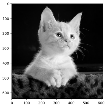
We can represent this image as a matrix:

from PIL import Image
import numpy as np

image = Image.open('cat.jpg')
gray = image.convert('LA')
image_matrix = np.array(list(gray.getdata(band=0)), float)
image_matrix.shape = (gray.size[1], gray.size[0])

Then we can perform singular value decomposition:

U, sigma, V = np.linalg.svd(image_matrix)

So far I have been describing these factorizations in terms of understanding linear transformations, but these help us understand data as well.

In the context of pixel data for an image, the SVD still tells us the same information it does for linear transformations. The singular values with the highest magnitudes correspond to the most important features of the matrix.

This image happens to be 612×640 pixels. So, $\Sigma$ would be a 612×640 diagonal rectangular matrix. Its columns have the largest singular values in order along the diagonal. The larger the value, the more that value explains our data.

So what would happen if we simply ignore the unimportant features of the data? We can truncate the matrices, leaving only the highest singular values and their corresponding singular vectors. Let’s say we keep the most important 200 singular values. We can reconstruct our image by simply multiplying the $U$ $\Sigma$ and $V$ together:

new_image = np.matrix(U[:, :200]) * np.diag(sigma[:200]) * np.matrix(V[:200, :]

Here’s what our new image looks like:

As you can see there is almost no perceptible drop in quality of the image, and yet the space needed to store our image has shrunk significantly.

We can try again, this time truncating even further:

new_image = np.matrix(U[:, :64]) * np.diag(sigma[:64]) * np.matrix(V[:64, :]

We’re starting to lose some quality at this point, but it is still very recognizably a cat.

SVD can clearly be used to apply lossy compression to an image, but it can do much more than that. This kind of compression could be applied to any data. Any media (music, video, etc.), or data matrix of any kind, can be compressed in a way that minimizes the loss of important features.

Principal Component Analysis

Data with many features is problematic. It takes more space to store in memory, takes more cycles to compute, and it is harder for us to interpret as humans.

Let’s consider the Iris data set. The Iris data set has 150 rows — 150 Iris plants. The columns of the data set are:

Sepal Length
Sepal Width
Petal Length
Petal Width

So, the entire data set is a 150×4 data matrix. We will call this data matrix $X$ .

Obviously, we can’t plot points in 4 dimensional space and interpret them graphically. We can, however do the same thing we just did for the image of a cat:

Perform Singular Value Decomposition
Reconstruct the original data at some lower dimensionality using our new singular values

Think about it: what are the chances that none of the features of a given data set are correlated? Putting it another way: how can we reduce the dimensionality of our data while preserving the maximum amount of information?

We could just go ahead and do SVD, but it’s actually not how PCA is done conventionally. Conventionally, PCA is done by eigendecomposing the covariance matrix. The covariance matrix is a symmetric matrix where each value along the diagonal corresponds to the variance of each feature, and the off-diagonal entries correspond to the covariance between the features:

$Cov(X, Y) = \dfrac{1}{n}\sum(X_i - \bar{X})(Y_i - \bar{Y})$

Because this blog post is about SVD I will explain why performing SVD on the original data and eigendecomposing the covariance matrix are mostly the same thing.

We want to reduce the dimensionality of the data in such a way that retains as much information as possible. If we perform SVD on the raw data set, the largest singular values will correspond to the “principal components” of the data.

Well, one important “hidden” feature of the data is the mean values of the features. We don’t really care about that, though. We want to capture variance. Graphically, subtracting the mean of the features from the data set will shift the data to the origin. The distances between the data points will not change. So, before doing singular value decomposition we will center our data about the mean:

Calculate the “mean vector”, $\mu$ . Each entry of this vector will be the mean of one of the features of our data set.
Subtract the $\mu$ from each row of our original data matrix, $X$

Now, with our data centered about the mean, we begin to perform SVD.

The first step in performing SVD is finding $X^TX$ .

Wait a minute…

Think about the calculations we’ve done so far:

Center the data about the mean
Multiply each row of $X^T$ by the corresponding column in $X$ and sum them together to get the entries of $X^TX$

That looks an awful lot like the formula above for covariance. The only thing missing is dividing by the number of rows in the data matrix. Indeed, $X^TX$ is a scalar multiple of the covariance matrix. It’s eigenvectors are the same. Dividing by the number of examples would give us the covariance matrix.

The next step in SVD is to eigendecompose. We’ve arrived at eigendecomposing the covariance matrix by another route.

Now that we have the eigenvectors of the covariance matrix we can project the original data onto the first $k$ eigenvectors. The number of eigenvectors we choose to keep is up to us. This is analogous to us choosing to truncate our matrix in the image compression example.

Let’s choose $k = 2$ principal components so that we can plot the data.

Here is the entire Iris data set plotted along its principal axes:

There is clearly structure to our data. There is an obvious separation between the points plotted on the left and on the right.

The Iris data set comes with a set of labels for each example, telling us what the actual species of Iris flower was. Coloring each point in the scatter plot according to its label gives us:

We have taken the data that was 4-dimensional and reduced it down to 2 dimensions. If we had a new Iris flower to plot we could measure its petal and sepal width/height, project it onto its principal axes to plot the point and see where it lands.

If it lands on the left we could be reasonably sure that it was an Iris-setosa (the purple dots).

Introducing a third eigenvector gives us a little more information, and we can still plot it in 3D:

There are clearly 3 distinct “slices” corresponding to each species of Iris flower.

The Moore-Penrose Pseudoinverse

I’ve saved the best for last. This is my personal favorite application of SVD.

In the first section of this blog post I discussed how matrices represent linear transformations. In the next sections I discussed how they also represent data. In this section I will talk about a third representation: systems of linear equations.

You may recall doing this from grade school math:

$2x + 1y = 10$

$3x - 3y = -4$

This system of linear equations can be solved with linear algebra. Here’s how:

First we add the coefficients of the variables into a matrix, $A$ :

$A = \begin{bmatrix} 2 & 1 \\ 3 & -3 \end{bmatrix}$

Next we put the solutions into a column vector, $b$ :

$b = \begin{bmatrix} 10 \\ -4 \end{bmatrix}$

The solution to this system can be found by solving for $x$ in the following equation:

$Ax = b$

There are a couple ways to proceed from here to solve this problem. One way is to multiply both sides of the equation by the inverse of the matrix $A$ , $A^{-1}$ :

$x = A^{-1}b$

The inverse, $A^{-1}$ of $A$ in this case is:

$A^{-1} \begin{bmatrix} 3/2 & -1/2 \\ -2 & 1 \end{bmatrix}$

$x = \begin{bmatrix} 3/2 & -1/2 \\ -2 & 1 \end{bmatrix} \begin{bmatrix} 10 \\ -4 \end{bmatrix} = \begin{bmatrix} 17 \\ -24 \end{bmatrix}$

That’s our answer. Go back and plug it into the original equation and see for yourself.

That’s all great, but the existence of an inverse depended on certain properties of $A$ :

It needs to be square
Its columns need to be linearly independent

This presents a problem because in reality a matrix is unlikely to have these nice properties.

If there are more equations (rows) than unknowns (columns) the system is overdetermined and equations can contradict each other leading to no solution. If the system has more unknowns (columns) than equations (rows) then the system is underdetermined and will have many possible solutions.

This is where the Moore-Penrose Pseudoinverse comes into play. The pseudoinverse is given by this equation:

$A^+ = V\Sigma^+U^T$

Where $V$ , $\Sigma$ , and $U$ are from the singular value decomposition of A. $\Sigma^+$ is the reciprocal of all of the non-zero elements of $\Sigma$ .

The pseudoinverse can be used in just the same way that we used the real inverse to solve a system of linear equations.

Even better, the solutions provided by the pseudoinverse are exactly what we hope they would be. The solution given by the pseudoinverse provides the solution which minimizes the Euclidean norm among all possible solutions. In other words, it is the line of best fit.

Let’s say we have some data:

x1 = [0, 50, 100, 150, 200, 250, 300, 350, 400, 450, 500] 
y = [0.13, 0.32, .4, .8, .8, 1.2, 1.12, 1.5, 1.6, 1.8, 1.9]

This could be any data. I will make up a story about this data and say that this is different pressure readings (ys) on a submarine at certain depths (xs).

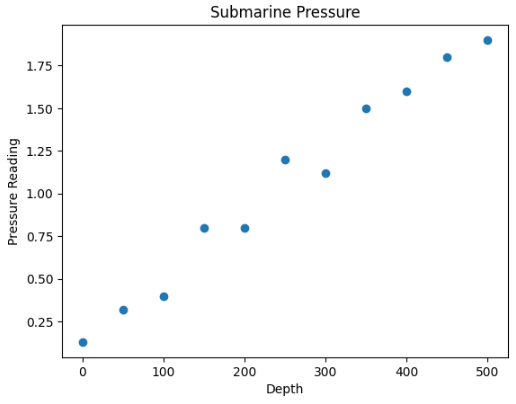
This system of linear equations has no linear solution. There is no straight line that one can draw that intersects all of these data points. The matrix representing this system of equations has no inverse. But it does have a pseudoinverse.

Finding the pseudoinverse and using it to solve this system of linear equations and plotting that solution gives us:

This is the line of best fit for our data. If we wanted to predict what the pressure reading would be at some other depth we could just plug it into this graph and see where we fall on the line.

The pseudoinverse can be used to solve otherwise unsolvable systems of linear equations of arbitrary size. This was a very simple 2-dimensional example, which yielded a line of best fit. At higher dimensionality the pseudoinverse would yield a “hyperplane of best fit”. It is a very powerful technique for modeling.

Conclusion

Diagonalizing a matrix can tell us a lot about the important features of that matrix. Singular value decomposition is a method for diagonalizing any matrix. For that reason it is a very powerful technique with many applications in data science and machine learning. It can be used to distill data down to its most important components, simplify a large data set, and build predictive models by solving unsolvable systems of linear equations.