Support Vector Machines From Scratch Part 2 – Optimizing the Margin

Introduction

This is the second installment in a series of blog posts about Support Vector Machines. If you have not read the first blog post, I highly recommend you go back and read it before continuing to this blog post.

Last time we looked at how to define the ideal hyperplane to linearly separate two classes of data. We ended up deriving this equation for the margin:

$\text{margin} = \dfrac{2}{\|w\|}$

The margin is the distance between the two closest points of each class. These two points are called the “support vectors”.

Optimizing the Margin

We want to maximize the margin to give ourselves as much breathing room as possible between the two classes. The margin is given by:

$\text{margin} = \dfrac{2}{\|w\|}$

Because the magnitude of the weight vector is in the denominator, we can increase the margin by lowering that magnitude.

This means that, mathematically, our optimization problem is simply:

$min \|w\|$

Subject to a few constraints:

All of the training data points in the positive class need to fall on or to the right of the positive support vector:

$y_i = 1 \rightarrow w^Tx_i - b \ge 1 \; \; \forall i_+$

And all of the points for the negative class must fall on or to the left of the negative support vector:

$y_i = -1 \rightarrow w^Tx_i - b \le 1 \; \; \forall i_-$

Because all of the $y$ s are either $1$ or $-1$ we can be clever and condense this down into one constraint by multiplying by $y_i$ :

$y_i(w^Tx_i - b) \ge 1 \; \; \forall i$

This problem is called the SVM primal. If you have encountered Support Vector Machines before, you may have also seen it in this form:

$min\dfrac{1}{2}\|w\|^2$

subject to:

$y_i(w^Tx_i - b) \ge 1 \; \; \forall i$

These are the same optimization problem. This form simply makes some of the math easier (hint: we will be taking derivatives). We will use this form going forward, but just know that is the same problem as the one we derived above.

Optimization Basics

Mathematical optimization techniques can help us find the maximum value or minimum value of a function.

Suppose we wanted to find the minimum of this function:

$x^2 - 8x + y^2 - 12y + 48$

In mathematical optimization, the function we want to optimize is called an objective function. You will sometimes hear it referred to as a loss function, especially in machine learning contexts.

I will write optimization problems with a $min$ or $max$ in front, depending on which kind of extremum we are looking to find:

$min x^2 - 8x + y^2 - 12y + 48$

Our goal is to find the values of $x$ and $y$ which produces the lowest possible value of our objective function. All we need to do is find the partial derivatives of the objective function, set them equal to 0, and solve.

First, we differentiate:

$\dfrac{\partial}{\partial x} = 2x - 8 = 0$

$\dfrac{\partial}{\partial x} = 2y - 12 = 0$

Solving for $x$ and $y$ :

$x = 4$

$y = 6$

We know for certain that these values for $x$ and $y$ give us a critical point of the function, a maximum or minimum, but we don’t know which it is. We can find out using the second derivative test. In this case, we have indeed found a minimum.

So can we use this technique to optimize the margin in the SVM primal? Unfortunately this by itself is not enough, because of the constraints. We will need more mathematical tools in our toolbox to solve this problem.

Lagrange Multipliers

Imagine we have a function:

$f(x, y)$

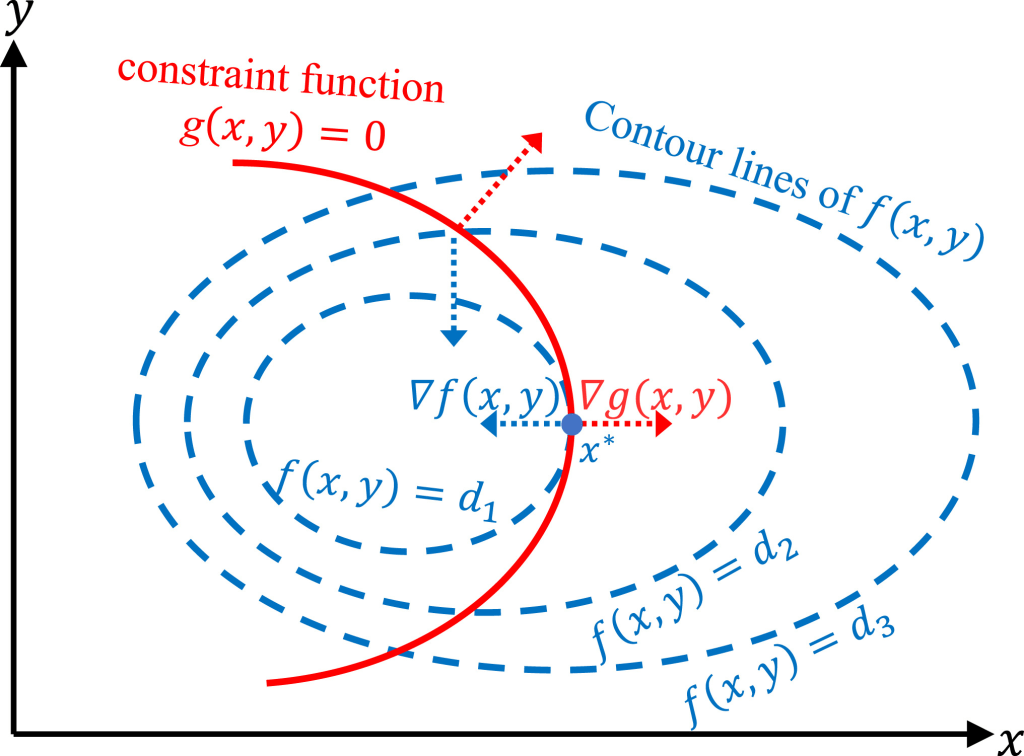
A two variable function is a surface. All along that surface are level curves (contour lines).

Now imagine we have a constraint:

$g(x,y) = c$

Where $c$ is some constant.

$g(x, y) = c$ is itself a level curve.

$f(x, y)$ and $g(x, y)$ are on the same plane. Therefore there is going to be some overlap between $g(x, y)$ and the level curves of $f(x, y)$ (if there is a solution).

The level curve for $g(x, y)$ is going to intersect a bunch of level curves of $f(x,y)$ . There is going to be one level curve of $f(x, y)$ that intersects at exactly one point.

The contour lines are either falling or rising. Where they intersect $g(x, y)$ at exactly one point must be an optimal point of the function subject to the constraint. It is either a minimum or a maximum.

At that point, the level curves will either have the same tangent or parallel tangents. This means that they will have normal vectors that are scalar multiples of each other (or exactly the same).

The vectors normal to these level curves are the gradient vectors of these curves.

This means that at a critical point of $f(x, y)$ this equality holds:

$\nabla f = \lambda \nabla g$

$\nabla f$ is the gradient of $f(x, y)$
$\nabla g$ is the gradient of $g(x, y)$
$\lambda$ is some scalar multiple

We call $\lambda$ a Lagrange multiplier.

Solving for this multiplier is relatively straightforward. Plugging this multiplier back into the equality will give us a critical point of the function.

Lagrange multipliers allow us to incorporate constraints into our optimization problem.

We can augment the original function, $f(x, y)$ to incorporate the equality constraint. This augmented form is called the Lagrangian and it looks like this:

$\mathcal{L}(x, y, \lambda) = f(x, y) - \lambda (g(x, y) - c)$

At first glance it may not be obvious the relationship the Lagrangian has to the equality $\nabla f = \lambda \nabla g$

If we were to optimize $\mathcal{L}(x, y, \lambda)$ we would find its gradient vector and set it to 0:

$\nabla \mathcal{L} = \begin{bmatrix} \dfrac{\partial \mathcal{L}}{\partial x} \\ \dfrac{\partial \mathcal{L}}{\partial y} \\ \dfrac{\partial \mathcal{L}}{\partial \lambda} \ \end{bmatrix} = 0$

So first let’s differentiate the Lagrangian with respect to $x$ :

$\dfrac{\partial \mathcal{L}}{\partial x} = \dfrac{\partial f}{\partial x} - \lambda \dfrac{\partial g}{\partial x}$

And now $y$ :

$\dfrac{\partial \mathcal{L}}{\partial y} = \dfrac{\partial f}{\partial y} - \lambda \dfrac{\partial g}{\partial y}$

Setting these equations equal to 0 to find the critical point we get:

$\dfrac{\partial f}{\partial x} = \lambda \dfrac{\partial g}{\partial x}$

$\dfrac{\partial f}{\partial y} = \lambda \dfrac{\partial g}{\partial y}$

This is just: $\nabla f = \lambda \nabla g$ written in component form. If we differentiate the Lagrangian with respect to $\lambda$ we get:

$\dfrac{\partial \mathcal{L}}{\partial \lambda} = g(x, y) - c$

Setting that equal to 0:

$g(x, y) -c = 0$

We just get our equality constraint back! This is to be expected. At the critical point the constraint must be satisfied.

Being able to rewrite a constrained optimization problem in the form of the Lagrangian is actually a huge win for us. We are essentially turning a constrained optimization (the original problem) into an unconstrained optimization problem (the Lagrangian) by incorporating the constraints directly into the problem. This allows us to optimize the Lagrangian with unconstrained methods we are familiar with (gradient descent for example) and get an optimal solution to the constrained problem.

If there were multiple constraints we would add a term for each constraint and its associated Lagrange multiplier. It is often written as a sum like this:

$\mathcal{L}(x, y, \lambda) = f(x, y) - \sum_{i = 1}^n(\lambda_i (g_i(x, y) - c))$

Where $n$ is the number of constraints. Since this is a sum of products you will also sometimes see this written in vector form as a dot product:

$\mathcal{L}(x, y, \lambda) = f(x, y) - \lambda^Tg$

This is still not quite enough firepower to solve the SVM primal problem. The constraints in the SVM problem are inequality constraints, and those are a bit more complicated.

Karush-Kuhn-Tucker Conditions

The Karush-Kuhn-Tucker approach expands upon the Lagrangian to incorporate inequality constraints into the function as well. It is sometimes referred to as the “Generalized Lagrangian” for that reason.

The Generalized Lagrangian looks like this:

$L(x, \lambda, \mu) = f(x) + \sum(\lambda_i g_i(x)) + \sum(\mu_j h_j(x))$

Note: whether you subtract or add the product of the constraints and the Lagrange multipliers to the original function is up to you. It does not change the optimal points. I’ve seen it more frequently written as an addition so I will use that form going forward.

The Lagrangian we looked at earlier is still there. We have also added on terms for the inequality constraints and their associated multipliers. In this formulation the $\lambda$ s are associated with the inequality constraints and the $\mu$ s are associated with the equality constraints. Technically, the multipliers on the inequality constraints are called KKT multipliers, but I’ve often just seen them all called Lagrange multipliers.

The basic idea behind the KKT approach is that, at the optimal solution, some of the inequality constraints will hold with strict equality. This means that they will act like equality constraints. These constraints are called active constraints. The inequality constraints that do not hold with strict equality are called inactive constraints.

If the inequality constraint is inactive, they may exclude potential optimal solutions, but an optimal solution with the constraint is still optimal if the constraint is removed. Their Lagrange multipliers should be set to 0.

The KKT approach lays out four conditions for optimality called the KKT conditions:

Stationarity Condition: $\nabla \mathcal{L} = 0$ . At an optimal point the gradient of the Lagrangian is 0.
Primal Feasibility: The solution must satisfy the original constraints.
Dual Feasibility The inequality constraints on the problem fall into two categories: active and inactive. Active inequality constraints are inequality constraints that are satisfied with strict equality at the optimal solution. Lagrange multipliers associated with active constraints must be non-negative. Inactive constraints should have a Lagrange multiplier of $0$ .
Complementary Slackness: Each inequality constraint must either have a Lagrange multiplier of $0$ , or the corresponding Lagrangian term is $0$ . In other words: $\sum_{i = 1}^n \lambda (g(x)) = 0$

SVM Dual

We can reformulate the optimization problem posed by the SVM Primal into a new form called the SVM dual.

Starting with the SVM Primal:

$min \dfrac{1}{2}\|w\|^2$

subject to

$y_i(w^Tx_i - b) \ge 1 \; \;\; \forall i$

We can get rid of the original inequality constraints by writing this in the Lagrangian form:

$\mathcal{L}(w, b, \alpha) = \dfrac{1}{2}\|w\|^2 -\sum \alpha_i(y_i(w^Tx_i - b) - 1)$

One important thing to note before we go any further is that there is one Lagrange multiplier $\alpha_i$ for each training example in our training data.

The dual formulation of the primal is the minimum of this function which maximizes the minimization problem posed by the Lagrangian.

$max_{\alpha}[min_{w, b}\mathcal{L}(w, b, \alpha)]$

In other words, the dual function is the smallest possible output of the Lagrangian over all possible values of $w$ and $b$ with some fixed values for the Lagrange multipliers, $\alpha$ .

Of course, the Lagrangian will be at a minimum when its derivative is 0. In other words, the gradient vector of the Lagrangian must be the zero vector.

So let’s differentiate the Lagrangian with respect to $w$ and $b$ :

$\dfrac{\partial L}{\partial w} = w - \sum_{i = 1}^n\alpha_iy_ix_i \rightarrow w = \sum_{i = 1}^n\alpha_iy_ix_i$

$\dfrac{\partial L}{\partial b} = \sum_{i = 1}^n\alpha_iy_i = \alpha^Ty = 0$

We can use these equations to solve for the optimal point of our Lagrangian. First, I will expand the summation in the Lagrangian:

$\mathcal{L}(w, b, \alpha) = \dfrac{1}{2}\|w\|^2 - w^T\sum \alpha_iy_ix_i - \sum\alpha_iy_ib + \sum \alpha_i$

Now, we can plug the equations for where the partial derivatives of $w$ and $b$ were zero into this equation:

$\mathcal{L}(w, \alpha) = \dfrac{1}{2}|w|^2 - w^Tw + \sum \alpha_i$

It is a fact about vectors that $w^Tw = \|w\|^2$ so this can be written as:

$\mathcal{L}(w, \alpha) = \dfrac{1}{2}\|w\|^2 - \|w\|^2 + \sum \alpha_i$

$\mathcal{L}(w, \alpha) = -\dfrac{1}{2}\|w\|^2 + \sum \alpha_i$

Again, plugging in our equation for $w$ we get:

$\mathcal{L}(\alpha) = -\dfrac{1}{2}\sum_{j=1}^n(\sum_{i=1}^n \alpha_iy_ix_{ij})^2 + \sum \alpha_i$

$\mathcal{L}(\alpha) = -\dfrac{1}{2}\sum_{i=1}^n\sum_{j=1}^n \alpha_i\alpha_jy_iy_j(x_i^Tx_j) + \sum \alpha_i$

$\mathcal{L}(\alpha) = \sum_{i = 1}^n\alpha_i - \dfrac{1}{2}\sum_{i=1}^n\sum_{j=1}^n \alpha_i\alpha_jy_iy_j(x_i^Tx_j)$

Therefore, our final dual formulation becomes:

$max \sum_{i = 1}^n \alpha_i - \dfrac{1}{2}\sum_{i = 1}^n \sum_{j = 1}^n \alpha_i \alpha_j y_i y_j(x_i^Tx_j)$

Subject to two constraints. The first constraint comes from the Dual Feasibility KKT condition, and it says that all of the Lagrange multipliers must be non-negative:

$\alpha_i \ge 0 \;\; \forall i$

The second constraint comes from the equation we got when finding the partial derivative of $b$ and setting it equal to 0 per the Stationarity Condition.

$\sum_{i = 1}^n\alpha_iy_i = 0 \;\; \forall i$

This is called the SVM Dual. It may not be immediately obvious in what way this form is superior to the primal. It looks more complicated!

For one, we’ve now rewritten our optimization problem in terms of only one decision variable. The SVM Primal is in terms of the weight vector $w$ and the bias term $b$ . The only unknowns in the dual form are the Lagrange multipliers $\alpha$ .

Truthfully, the biggest reasons to use the dual form as opposed to the primal I have not covered yet, namely kernels and SMO. We will get there when we get there, but for now you should familiarize yourself with the SVM dual, because it is the function we will be dealing with for the rest of this series.

Conclusion

This was a pretty theory-heavy post. It was mostly a crash-course in optimization, covering the techniques we will need to train an SVM. In the next blog post we will get hands on, and use the SVM Dual formulation to train an SVM from scratch.

Thank you for reading!