Support Vector Machines From Scratch Part 5 – Kernels

Introduction

This is the fifth installment in a series of blog posts about Support Vector Machines. If you have not read the four other blog posts, I highly recommend you go back and read those before continuing to this blog post.

Last time we introduced soft-margin SVM, which was a new formulation that could accommodate data that was not perfectly linearly separable. Soft-margin SVM makes SVMs much more applicable to real data because real data is often noisy.

What about data that is not linearly separable at all? Believe it or not, we can use SVMs to classify data that is not linearly separable. In this blog post, we will discuss our means of doing so: kernels and the kernel trick.

Nonlinear Data

Imagine our data looked like this:

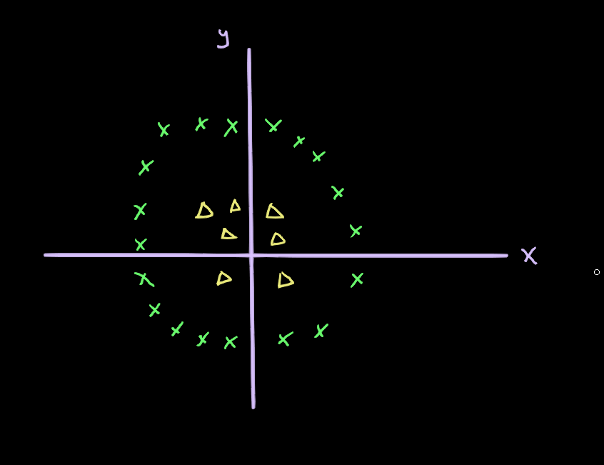
Although there is a separation between the two classes, there is no linear separation. We can’t draw a straight line that separates the data points into two classes.

What if we add an extra dimension to the data, though? Let’s add a third dimension to each data point. The value of the third dimension will just be derived from the existing dimensions. Let’s call this point $z$ . $z$ will be $x^2 + y^2$ .

Now, plotting our data we get:

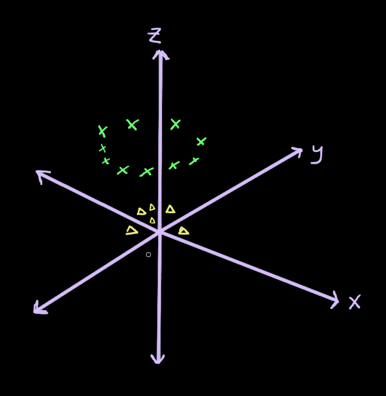
As you can see, because the values of the yellow triangles were smaller before (closer to the origin) they are going to be lower on the $z$ axis. The green xs had larger values so they are going to be higher on the $z$ axis.

Now our data is linearly separable. We can draw a hyperplane (in this case a 2-dimensional plane) which separates the two classes:

Mapping Up to Higher Dimensions

Suppose our data was 2-dimensional. Each training example, $x$ , would be represented as a 2-dimensional vector:

$x = \begin{bmatrix} x \\ y \end{bmatrix}$

We could map this vector up to a higher dimensional space, using the features that already exist, by using all of the possible 2nd-degree combinations of the features. We’ll call this vector $\phi$ :

$\phi = \begin{bmatrix} 1 \\ x \\ y \\ x^2 \\ y ^2 \\ xy \end{bmatrix}$

That’s six possible combinations. We’ve mapped our 2-dimensional data up to 6 dimensions.

So, why don’t we just do this?

Mapping a 2-dimensional vector up to 6-dimensional space may not be so bad, especially for only one training example, but with higher dimensional data and lots of training data, this quickly becomes intractable.

The SVM Dual

Let’s take a look at the dual formulation real quick and see how this mapping of our data into higher dimensions might affect our calculations:

$max \sum_i\alpha_i - \dfrac{1}{2}\sum_i\sum_j\alpha_i\alpha_jy_iy_j(x_i^Tx_j)$

As you can see, the only place our feature vectors come into play is the:

$x_i^Tx_j$

We’re taking the dot product of two of our feature vectors.

So, if we started with 2-dimensional data, but mapped it up to 6-dimensional data as described above, each of these dot products would look like this:

$\phi_i^T\phi_j = \begin{bmatrix} 1 & x_i & y_i & x^2_i & y^2_i & x_iy_i \end{bmatrix} \begin{bmatrix} 1 \\ x_j \\ y_j \\ x^2_j \\ y^2_j \\ x_jy_j \end{bmatrix}$

$\phi_i^T\phi_j = 1 + x_ix_j + y_iy_j + x^2_ix^2_j + y^2_iy^2_j + x_ix_jy_iy_j$

In summary:

We mapped our 2-dimensional data up to 6 dimensions by finding all of the 2nd degree combinations of the features.
We took the dot products of two of these feature vectors.

The problem arises from step 1. Mapping the original feature vectors up to higher dimensions can require so much memory as to be impractical.

What if we could go about this another way? What if we designed a clever function that produced the same result as the dot product of our 6-dimensional feature vectors?

Consider this function:

$K(x_i, x_j) = (1 + x_i^Tx_j)^2$

Recall our original feature vectors:

$x_i = \begin{bmatrix} x_i \\ y_i \end{bmatrix} \;\; x_j = \begin{bmatrix} x_j \\ y_j \end{bmatrix}$

Taking the dot product of these two gives us:

$x_i^Tx_j = x_ix_j + y_iy_j$

Plugging this into our function:

$(1 + x_ix_j + y_iy_j)^2$

And then we distribute and get:

$1 + x_ix_j + y_iy_j + x^2_ix^2_j + y^2_iy^2_j + x_ix_jy_iy_j$

This is exactly what we got when we took the dot product of $\phi_i$ and $\phi_j$ (our 6-dimensional feature vectors).

As you’ve probably guessed $K(x_i, x_j)$ is a kernel function. There are many kinds of kernel functions. This one is called the polynomial kernel function.

The fact that $K(x_i, x_j) = \phi_i\phi_j$ is huge.

This means that we can effectively get the benefits of mapping our data up to 6-dimensional space simply by replacing: $x_i^Tx_j$ in the dual with $K(x_i, x_j)$ .

$max \sum_i\alpha_i - \dfrac{1}{2}\sum_i\sum_j\alpha_i\alpha_jy_iy_jK(x_i, x_j)$

This is what’s called the kernel trick. We do not need to map our data up to 6 dimensions. We do not need any more storage to store our data. It almost feels like cheating.

There are many other kernel functions that we may go over in detail later. One of the most interesting ones is called the radial basis function kernel (or Gaussian kernel) which maps your data up to infinite dimensions. This would be impossible without the kernel trick, but with the kernel trick, it’s no big deal. You just plug your feature vectors into this function:

$K(x_i, x_j) = e^{-\dfrac{\|x_i - x_j\|^2}{2}}$

Conclusion

At this point we’ve covered most of the fundamental theory behind Support Vector Machines at a high level. In the next blog post, we will be circling back to our implementation in Python. We will take a look at a method for training SVMs that is superior to the QP solver solution we saw in the third blog post: Sequential Minimal Optimization.

Thank you for reading!