Introduction
This is the sixth installment in a series of blog posts about Support Vector Machines. If you have not read the first five blog posts, I highly recommend you go back and read those before continuing on to this blog post.
Last time we looked at kernels and the kernel trick, which allowed us to use SVMs to classify data that is not linearly separable.
In this blog post we will be focusing once again on how we train SVMs. In the third blog post I introduced Quadratic Programming and we used the CVXOPT QP solver in Python to train our SVM.
In this blog post I will be describing in detail a superior algorithm specifically designed for training Support Vector Machines called Sequential Minimal Optimization (SMO).
Sequential Minimal Optimization is a modified version of an optimization algorithm called coordinate ascent. In SMO, we solve the optimization problem posed by the SVM dual iteratively by solving the smallest possible optimization subproblem at every step.
Why Sequential Minimal Optimization?
Why do we even need SMO? We were already training our SVM without it, after all.
It is true that we can train SVMs using Quadratic Programming solvers such as CVXOPT. As a matter of fact, until SMO’s discovery/invention by John Platt in 1998, QP solvers were how SVMs were trained. There are many issues with QP solvers, though.
First of all, QP solvers are notoriously tricky to implement. There are many numerical precision issues and things like that to deal with. SMO is quite straightforward to implement. We will be implementing the algorithm ourselves from scratch.
Also, the techniques that QP solvers use to actually train SVMs involve keeping very large matrices in memory, and performing computationally costly operations with them. In the toy examples we looked at, you likely wouldn’t have run into any issues, but in a real scenario you could very easily hit a wall with large data sets where QP solvers are simply too inefficient to get the job done. SMO, on the other hand, does not require any of these expensive matrix operations whatsoever.
Coordinate Ascent
Coordinate ascent is an algorithm for maximizing objective functions.
The algorithm goes like this:
- Start with an initial guess at what the variables should be.
- Pick one decision variable.
- Find the partial derivative of the objective function with respect to that variable.
- If the partial derivative with respect to that variable is 0, pick another variable. If the partial derivative with respect to all variables is 0, you’ve found the maximum.
- Step that variable in the direction of that partial derivative, keeping the other decision variables constant.
- Repeat from step 2 until you’ve found the maximum.
Let’s take a look at one of the examples we saw in the second blog post:

This is a minimization problem. Coordinate ascent is for maximizing objective functions.
I’d like to change this minimization problem into an maximization problem so that, if we successfully perform coordinate ascent, we will get the same answer we did in the second blog post. To do this we just need to negate the objective function.

Alternatively, we could modify the algorithm slightly to step the decision variable in the opposite direction of the partial derivative. This is called coordinate descent, and it would minimize our objective. For the sake of relating this to SMO, we will stick with coordinate ascent.
Now, we start by picking an initial guess at our decision variables (


Let’s start by optimizing
We find the partial derivative of our objective with respect to

We plug in our current value of 
Now we need to step our current value of 
So we increase
Now we repeat the process with 
Graphically, coordinate ascent looks like this:
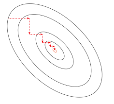
The ellipses are the contour lines of our function. The red lines represent the steps we take in the direction of
Sequential Minimal Optimization
So, can we use coordinate ascent to optimize the SVM dual?
Recall that the SVM dual is:

subject to:

Unfortunately, we can’t. The reason we can’t is the linearity constraint:
This means that all of the Lagrange multipliers lie on a line. Each 

To get around this, SMO uses a modified version of coordinate ascent where we solve for two Lagrange multipliers at a time.
Derivation
This section is a full derivation of the solution for one iteration of SMO’s modified version of coordinate ascent. I could not find the full derivation anywhere online so I feel compelled to post it in its entirety, step by step. The original paper has a derivation, but it skips over a lot.
If you do not care about the derivation you can skip this section. If you see any issues in my derivation please let me know.
Our goal is to optimize the SVM dual by solving for two Lagrange multipliers at a time.
Looking at the linearity constraint:

We can rewrite it to be in terms of 


The term on the right-hand side is just some fixed constant that we can calculate. We will call this constant 

We can now solve this equation for

Since 


Distributing the

Now, I would also like to make a substitution in this equation using this equality:

Plugging this back into the equation for

Now we can rewrite the dual in terms of

This looks very complicated, but all I have done is separate the terms in the summation that include
Now, we can reformulate this equation into being in terms of only 

Now, I will introduce another variable to help simplify this equation:

Plugging 

Now we have the dual equation in terms of only two Lagrange multipliers. This is still a Quadratic Program. We could plug this into a QP solver and it would still be much faster than before overall because we only have two decision variables.
We can do even better though, and solve for
To analytically solve for
Let’s differentiate it term by term:
First Term: 
We differentiate this with the chain rule and get:

Second Term: 
We use the power rule:

Third Term: 
Here we just apply the constant rule and get:

Fourth Term: 
First, we distribute the 

Next, we distribute the

Therefore:

But, recall that 

Because 


Fifth Term: 
This is a straightforward application of the constant rule:

Sixth Term: 
First, we distribute the negative:

Then apply the constant rule:

Seventh Term:
This is obvious:

Eighth Term:
The eighth term is a constant that does not include
At long last putting the terms together into one equation and setting that equation equal to zero gives us:

Now, we need to solve for
First, we can move 

Now we can factor a 

Wherever there is parenthesis on the left side of the equation we can distribute:

Since 

Combining like terms:

We can factor out the 

We can factor out the

At this point we need to take another look at the equation for
Solving for

We don’t know what

Where the starred variables are the values found in the previous iteration.
Plugging this equation in for

Distributing some of the parenthetical terms out on the right side of the equation gives us:


Now, to make further progress we must revisit the equation we had for

Defining a new variable, 


We can solve 

Once again this is in terms of the values from the previous iteration (our current parameters).
Plugging this equation for

The 

We can distribute the 


Now we have some terms that cancel out:

We can group all of the terms containing 

And factor out a

Now we can factor out a

Notice how
Now, I will define another variable:

And substitute into the equation:

Now we divide both sides by 

The original paper defines another variable:

which is the “error” in the
Rewriting our equation in terms of 

Which is the equation found in the paper.
Keeping The Solution Feasible
There is one more step,
This is the analytical solution for
All we need to do to obey these constraints is to clip our
For example, we know from the linearity constraint:
Solving this equation for
We know that all of the
There are two possibilities:


Let’s first take a look at the case where 
We can plot this line to help gain some intuition about how we need to clip

A solution which satisfies the linearity constraint must lie on the diagonal line:

As you can see when the line crosses the 

When 

The same is true of the other end of the line segment when 
Not only must our solution lie on this line, but it must also lie within a box because of the inequality constraints: 
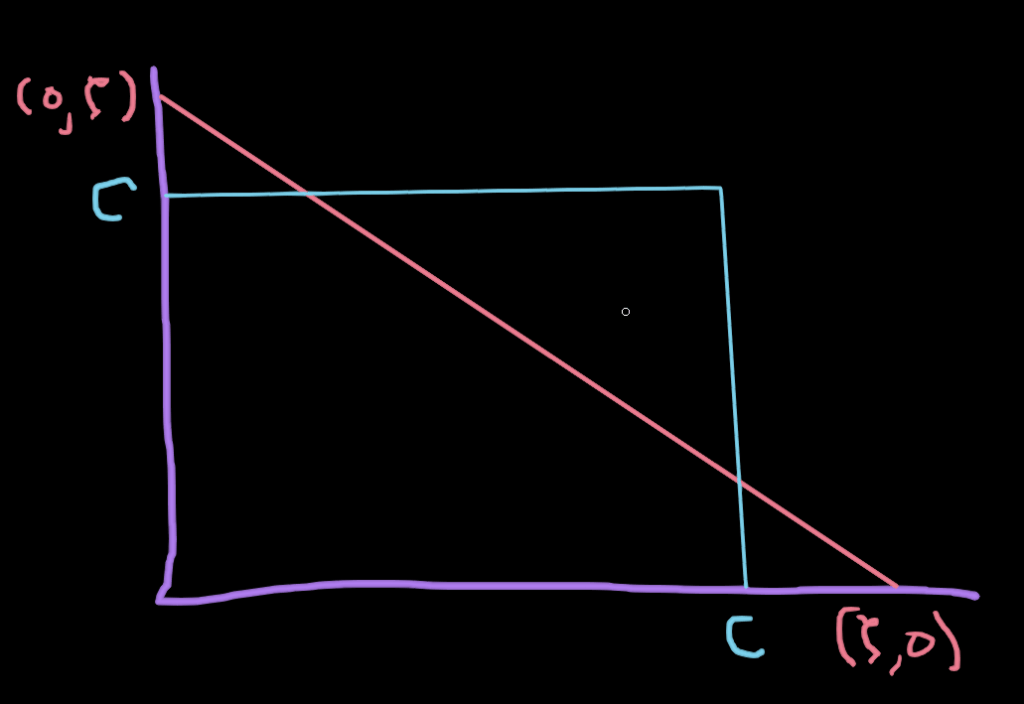
If we let ![[0, C]](https://s0.wp.com/latex.php?latex=%5B0%2C+C%5D&bg=ffffff&fg=000&s=0&c=20201002)


We can define the bounds like this:


Plugging back in the equation for


If the labels are not equal to each other: 


Now, the bounds look like this:


Again, writing these bounds in terms of


That’s it. We can now solve for two Lagrange multipliers at a time in the dual problem, keeping the solution feasible at every step.
Conclusion
To recap the algorithm it goes like this:
- Select two Lagrange multipliers,
- Solve for
- Clip this solution for
- Repeat until convergence.

There is a whole other component of the algorithm that the paper goes into which is heuristics for choosing which Lagrange multipliers to optimize, but we can just select them at random and it may still converge. I will put that off until later for now, and jump into the simplest possible implementation of SMO.
Thank you for reading!

Leave a comment