Introduction

In a previous series of blog posts I covered feedforward neural networks. Feedforward neural networks are very powerful, but they are not the only neural network architecture available and they may be ill-suited to certain tasks.

Recurrent neural nets are a class of neural nets that are particularly effective for modeling data with a sequential topology, e.g. stock prices, weather data and language. Language is what I will be focused on in these blog posts. I will be building a simple recurrent neural net from scratch to generate fake names.

I will try to assume as little prior knowledge as possible during this series, but if you are not familiar with feedforward neural networks or basic neural network concepts, I would recommend reading my series on feedforward networks first. I will be focusing on building an intuition and implementation of recurrent neural networks from scratch, and will not be using any machine learning libraries.

Why Recurrent Neural Nets?

Let’s say we want to train a neural network to extract the year in a given sentence.

For example, consider these two sentences:

1. The Mets won the World Series in 1986.
2. In 1986, the Mets won their second World Series.

There are three main characteristics of a feedforward neural net that make accomplishing this task difficult:

1. A feedforward neural network only has connections that go forward. There are no recurrent connections, i.e. connections within the same layer, or connections that go backward.
2. The inputs must be of a fixed size.
3. A feedforward neural network has separate parameters (weights/bias) for each neuron.

These characteristics make it difficult to process inputs of varying length, learn position-independent feature extracting rules, or leverage context from different positions in the sentence.

A recurrent neural net is a network that does away with these restrictions to achieve better performance on tasks like this.

Recurrent neural nets:

1. Have recurrent connections, allowing them to not only process sequences of arbitrary length, but also to build up a kind of memory about previous inputs to the network.
2. Share parameters, allowing the network to learn to extract features irrespective of their position in the sequence.

That all sounds great, but how exactly do we structure a neural network that has recurrent connections?

It may seem like a daunting task at first glance, but it’s actually quite simple. If we think about our network in terms of its computation graph, a recurrent neural network is really a dynamic sequence of connected feedforward neural networks.

Computation Graphs

A computation graph is a directed graph that models a computation. Computation graphs are useful in many neural network contexts. We briefly looked at computation graphs in the feedforward network series when we talked about backpropagation. Computation graphs are essential to understanding recurrent neural networks.

Dynamical Systems

Consider a dynamical system:

• is the “state” of the system at time step
• is a function that transitions from the previous state

It’s computation graph looks like this:

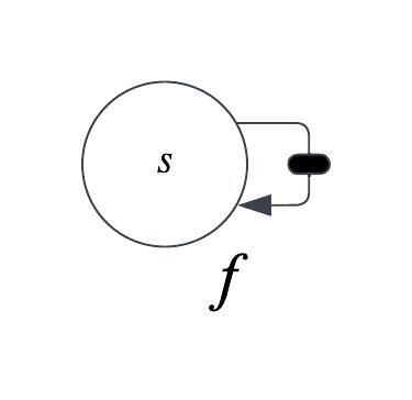
The looped arrow indicates a recurrent connection. The black box indicates a delay of one time step. We move from one time step to the next by applying the function .

For a finite number of time steps, we can unfold this computation graph:

For example, if we have three timesteps:

The unfolded computation graph looks like a standard directed acyclic graph. There are no more recurrent connections:

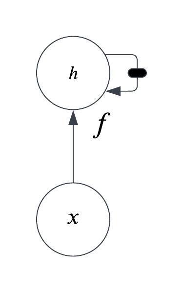
Dynamical Systems with an External Signal

Now we will add one more feature to the system: an external signal.

The equation for our system with an added external signal that influences the state is:

• is the “state” of the system at time step
• is a function that transitions from the previous state to the next state, as before. Now it is a function of the external signal at timestep , as well as the previous state of the system

Here is the computation graph:

Once again, if we have a finite number of time steps we can unfold this computation graph:

This is the fundamental structure of a recurrent neural network.

Here is the computation graph for the recurrent neural network I will be building:

• is the hidden state at the time step
• is the input at timestep
• is the output at timestep
• is the weight matrix connecting the inputs to the hidden layer neurons.
• is the weight matrix connecting the hidden layer neurons to the output neurons.
• is the weight matrix connecting the previous hidden state to the next hidden state. Much like the same function mapped previous states to future states, the same weight matrix is used to map previous states to future states.

The hidden nodes on the graph with dotted lines are there to indicate that this unfolded computation graph could be arbitrarily long. It does not necessarily need to be three time steps long.

Unfolding computation graphs with recurrent connections allows us to achieve the goals we stated in the introduction of this post, i.e. processing sequences of arbitrary length and parameter sharing:

1. Because the graph is defined in terms of the transition from one state to the next, we can easily process sequences of varying length by simply processing one state after another. The only thing we need to compute the next state is the value of the previous state.
2. The same function is used to transition between states at each step, which uses the same parameters.

becomes a kind of lossy summary of all past states. If the capacity of the network is sufficient, we can model complicated sequences of arbitrary length using the same function for transitioning from one sequence to the next.

Conclusion

Hopefully this blog post has given you some intuition about how a recurrent neural network is structured, and why it is so good at sequence processing tasks.

In the next blog post we will look at the data our recurrent neural network will be trained on, and begin the implementation of our recurrent neural net.

Thank you for reading!