Introduction

In the previous blog post we talked about what it means exactly for data to have a “sequential topology”, and prepared our training data to be fed into the recurrent neural net.

In this post, we’ll be looking at the design of our simple recurrent neural net, the equations for the forward pass, and finally begin implementing our neural net in code.

The Forward Pass

To start things off, it’s worth taking a look again at the unfolded computation graph for our network:

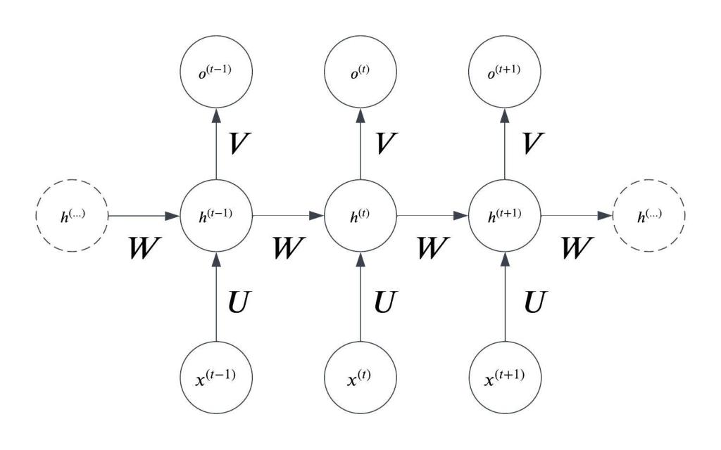
As we talked about in the first post, this is essentially a dynamically constructed sequence of feedforward neural nets where the hidden state from the previous timestep is fed back into the hidden layer of the current timestep.

We will continue doing this in a loop until we have reached the end of the sequence.

The outer loop for the forward pass will look like this:

for i in range(input.shape[0]):
    output, hidden = rnn.forward(input[i], hidden)

The implementation of the forward() function is quite similar to how you would implement the forward pass of a feedforward network. The only difference is that the previous hidden state is taken into account.

The design of the recurrent neural net I will be building will be very simple:

1. A linear layer connecting the inputs to the hidden layer.
2. A hyperbolic tangent nonlinearity after the hidden layer.
3. A linear layer connecting the hidden units to the outputs.
4. A softmax will be applied to the outputs so that we can interpret the output vector as a probability distribution.

In terms of parameters, this means we will need the following:

1. : the weight matrix connecting the input to the hidden layer.
2. the bias vector associated with the first hidden layer.
3. the weight matrix connecting the hidden units to each other.
4. the weight matrix connecting the hidden layer to the output layer.
5. the bias vector associated with the output layer.

Note that these parameters are “shared” in the sense that they are the same for each time step.

With this in mind we can begin implementing our RNN class:

class RNN():
    def __init__(self, input_size, hidden_size, output_size):
        self.input_size = input_size
        self.hidden_size = hidden_size
        self.output_size = output_size
        
        self.U = np.random.randn(hidden_size, input_size)
        self.W = np.random.randn(hidden_size, hidden_size) 
        self.V = np.random.randn(output_size, hidden_size) 
        self.b = np.random.randn(hidden_size)
        self.c = np.random.randn(output_size)

The Forward Propagation Equations

Before we begin implementing the forward pass, I need to lay out the equations.

The first layer is simple enough:

This is the contribution to the hidden state from the input, but there is another component: the previous hidden state:

Putting it together, the weighted sum for the hidden layer is:

We pass this weighted sum through a hyperbolic tangent activation function to get our final hidden layer activation value:

Now, to get our output for this timestep, we pass our hidden layer activations through another linear layer:

And finally, to get our output activations we apply a softmax function:

This translates to code pretty directly. The important thing to note here is that we return the output and the value of the hidden state for that timestep. That value will be fed into the forward pass of the next timestep.

class RNN():
    def __init__(self, input_size, hidden_size, output_size):
        self.input_size = input_size
        self.hidden_size = hidden_size
        self.output_size = output_size
        
        self.U = np.random.randn(hidden_size, input_size)
        self.W = np.random.randn(hidden_size, hidden_size) 
        self.V = np.random.randn(output_size, hidden_size) 
        self.b = np.random.randn(hidden_size)
        self.c = np.random.randn(output_size)

    def forward(self, input, hidden):
        z_t = self.b + self.W @ hidden + self.U @ input
        h = np.tanh(z_t)
        a = self.c + self.V @ h
        o = softmax(a)
        return o, h

That’s all we need in terms of the forward pass. I have also defined a helper function:

def init_hidden(self):
    return np.zeros(self.hidden_size)

Which returns the initial hidden state (all zeros).

And another helper function, that does not belong to the RNN class, for computing the softmax:

def softmax(z):
    # Numerical stability: subtract max value from z
    z_max = np.max(z)
    z_exp = np.exp(z - z_max)
    norm_constant = np.sum(z_exp)
    result = z_exp / norm_constant
    return result

The full outer loop of the forward pass looks like this:

hidden = rnn.init_hidden()
input = inputs[0]
os = np.zeros((input.shape[0], rnn.output_size))
hs = np.zeros((input.shape[0], rnn.hidden_size)) 
    
for i in range(input.shape[0]):
    output, hidden = rnn.forward(input[i], hidden)
    os[i] = output
    hs[i] = hidden

Conclusion

In this blog post we looked at the forward pass through a recurrent neural net, and implemented our RNN class in Python. Hopefully this helped cement the ideas of how a recurrent neural network works, and how it is different from a feedforward neural net.

In order to train our neural net, we will need to perform backpropagation to obtain the gradients we will use to update our parameters. In the next blog post I will be going over the backpropagation through time algorithm in detail, deriving the equations for backpropagation from the forward propagation equations, and explain how the gradients propagate through time.

Thank you for reading!