Recurrent Neural Networks From Scratch Part 4 – Backpropagation Through Time

Introduction

In the previous blog post, we began the implementation of our feedforward neural net, and went over the equations and code for the forward pass.

With this, we can now feed our data through the network, but its not of much use without being able to train it. In order to train our recurrent neural network, we need to implement the backpropagation through time algorithm.

If you have not read my blog post on the basics of backpropagation, I highly recommend you read that (and the rest of the feedforward neural net series) before reading this blog post.

Loss Function

Before we can begin training our neural net we need a way of measuring how well our network is actually performing, i.e. a loss function.

We will be using a negative log loss function. This choice is motivated mainly by the fact that our problem is a classification problem (“which character comes next?”), and our output layer, being softmax, represents a probability distribution.

Any choice of loss function would work in principle, but the equations I will be deriving are specifically for the network discussed in the last blog post, and a negative log loss function.

Negative log loss looks like this:

$L = -log(\hat{y}^{(t)}_{y^{(t)}})$

$\hat{y}^{(t)}$ is the full output vector from the softmax output layer for time step $t$ . Each element represents a probability (between 0 and 1) that the output is of the class associated with that element in the vector.
$\hat{y}^{(t)}_{y^{(t)}}$ is the element of the full output vector associated with the true label value.

Note that this is the loss for a single timestep. The total loss for the whole sequence can be computed in different ways. Simply summing the losses for each time step, or taking an average are both valid. We’ll be summing them.

loss = 0

for t, (y_hat, target_seq) in enumerate(zip(os, target)):
    target_index = target_seq.argmax().item()
    loss += -np.log(y_hat[target_seq.argmax().item()])

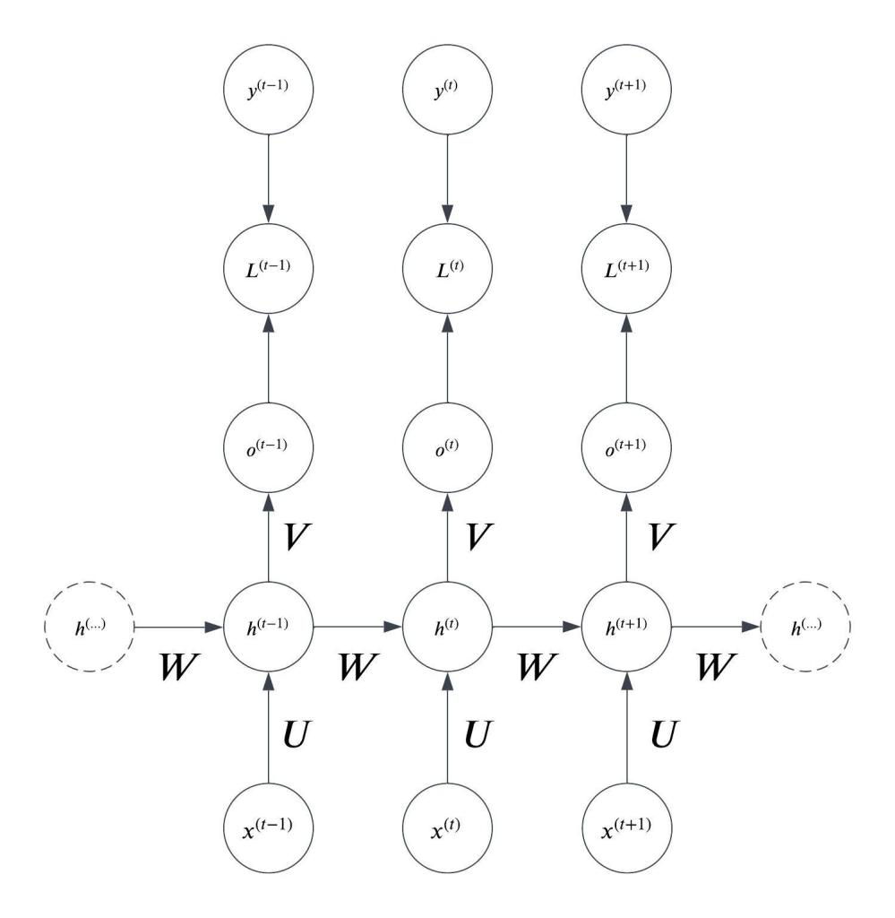
Our computation graph now includes the nodes for the loss at each timestep, with the output of the neural net and the true label value as inputs:

Our goal is to drive this loss function as low as possible during training. To do that, we need to compute the gradient of the loss with respect to the parameters.

Backpropagation Through Time

The basic idea of the backpropagation through time algorithm is that, once we have the unfolded computation graph laid out before us, we can backpropagate through it as though it were one long connected feedforward neural net.

While each node in the computation graph above actually represents an entire layer of neurons, I will be making the simplifying assumption during much of this derivation that each layer is in fact only one neuron large.

I find this helpful for understanding how the equations are derived, and it’s not difficult to generalize to the matrix/vector case afterwards.

Starting from the loss node for the final time step in the computation graph we work recursively backwards, computing the gradient of each node with respect to the loss using the chain rule.

Autograd engines like the one in PyTorch actually construct this computation graph automatically behind the scenes when you do operations with tensors. When you call .backward(), it backpropagates through that computation graph automatically. This is especially helpful in recurrent neural nets because it means that you don’t need to keep the hidden states around for training. This being from scratch, we will be implementing the backpropagation by hand.

The first node (the loss itself) is obvious:

$\dfrac{\partial L}{\partial L^{(t)}} = 1$

Output Layer

The next step is to find the partial derivative of the loss with respect to the output at each timestep.

To do this we use the chain rule:

$\dfrac{\partial L}{\partial o_i^{(t)}} = \dfrac{\partial L}{\partial L^{(t)}}\dfrac{\partial L^{(t)}}{\partial o_i^{(t)}}$

Since $\dfrac{\partial L}{\partial L^{(t)}} = 1$ this simplifies to just:

$\dfrac{\partial L}{\partial o_i^{(t)}} = \dfrac{\partial L^{(t)}}{\partial o_i^{(t)}}$

Now, to find the derivative of the loss for time step $t$ with respect to the output we need to use the chain rule again and find:

$\dfrac{\partial L^{(t)}}{\partial o_i^{(t)}} = \dfrac{\partial L^{(t)}}{\partial \hat{y}^{(t)}} \dfrac{\partial \hat{y}^{(t)}}{\partial o_i^{(t)}}$

First we differentiate the loss function with respect to $\hat{y}$ :

The loss function is:

$L = -log(\hat{y}^{(t)}_{y^{(t)}})$

$\dfrac{\partial L^{(t)}}{\partial \hat{y}^{(t)}} = \dfrac{1}{\hat{y}^{(t)}_{y^{(t)}}}$

Now we find the partial derivative of $\hat{y}$ with respect to the output:

Recall that the output is softmax:

$\hat{y}_i = \dfrac{\text{exp}(o_i)}{\sum_j\text{exp}(o_j)}$

To find: $\dfrac{\partial \hat{y}_i}{\partial o_i}$ we need to use the quotient rule:

$\dfrac{\partial \hat{y}_i}{\partial o_i} = \dfrac{exp(o_i)\sum_j\text{exp}(o_j) - exp(o_i)exp(o_i)}{(\sum_j\text{exp}(o_j))^2}$

$\dfrac{\partial \hat{y}_i}{\partial o_i} = \dfrac{exp(o_i)(\sum_j\text{exp}(o_j) - exp(o_i))}{(\sum_j\text{exp}(o_j))^2}$

We can separate this fraction out:

$\dfrac{\partial \hat{y}_i}{\partial o_i} = \dfrac{exp(o_i)}{\sum_j exp(o_j)} \times \dfrac{\sum_j o_j}{\sum_j o_j} - \dfrac{exp(o_i)}{\sum_j exp(o_j)}$

Simplifying and plugging in our equation for $\hat{y}$ :

$\dfrac{\partial \hat{y}_i}{\partial o_i} = \hat{y}_i(1 - \hat{y}_i)$

And finally we return to this equation:

$\dfrac{\partial L^{(t)}}{\partial o_i^{(t)}} = \dfrac{\partial L^{(t)}}{\partial \hat{y}^{(t)}} \dfrac{\partial \hat{y}^{(t)}}{\partial o_i^{(t)}}$

$\dfrac{\partial L^{(t)}}{\partial o_i^{(t)}} = -\dfrac{1}{\hat{y}^{(t)}_{y^{(t)}}} \hat{y}_i(1 - \hat{y}_i)$

$\dfrac{\partial L^{(t)}}{\partial o_i^{(t)}} = \hat{y}^{(t)}_i - 1_{i,y^{(t)}}$

Where the $1$ is just an indicator function. It is a $1$ in the element where the true label value is $1$ and a zero everywhere else (in other words, our one-hot encoded target vector).

With this, we can begin implementing the backpropagation for our RNN class:

def backward(self, input, target, outputs, hs):
    time_steps = len(input)
        
    # Output layer
    dLdots = [np.zeros(self.output_size) for _ in range(time_steps)]
    for t in range(time_steps):
        dLdot = outputs[t] - target[t]
        dLdots[t] = dLdot

Hidden Layers

For the hidden layer associated with the final timestep, $\tau$ , the backpropagation is simple. It is the same as it would be in a normal feedforward scenario with a single hidden layer.

Note that in this case $h^{(\tau)}$ is the activation value of the hidden layer, not the weighted sum.

Therefore, the gradient for this layer is:

$\dfrac{\partial L}{\partial h^{(\tau)}} = \dfrac{\partial L}{\partial o^{(\tau)}} \dfrac{\partial o^{(\tau)}}{\partial h^{(\tau)}}$

We computed $\dfrac{\partial L}{\partial o^{(\tau)}}$ in the last section so we just need to find $\dfrac{\partial o^{(\tau)}}{\partial h^{(\tau)}}$ :

Recall that when we feed the activations of $h^{(\tau)}$ forward, we pass them through the weight matrix $V$ :

$o^{(\tau)} = Vh^{(\tau)}$

Therefore:

$\dfrac{\partial o^{(\tau)}}{\partial h^{(\tau)}} = V^T$

In our simple one-neuron-per-layer example, this would just be a scalar number and transposing it makes no sense. In a real scenario though $V$ would be a full matrix.

Putting it all together we get:

$\nabla_{h^{(\tau)}}L = V^T\nabla_{o^{(\tau)}}L$

Backwards Through Time

Given the gradient of the hidden layer for the final time step $\tau$ , we can propagate backwards through time.

In the previous section, we found the gradient of the hidden layer of the final timestep. We want to find $\nabla_{h^{(t)}}L$ for each hidden layer before the final hidden layer.

There are two descendants of $h^{(t)}$ in the computation graph that will contribute to its gradient: $h^{(t + 1)}$ and $o^{(t)}$ .

We already know $\nabla_{h^{(t + 1)}}L$ and $\nabla_{o^{(t)}}L$ . We showed how to calculate those above. $\nabla_{h^{(t + 1)}}L$ is either the gradient of the final hidden layer $h^{(\tau)}$ or the hidden layer you last computed the gradient for.

$\dfrac{\partial L}{\partial h^{(t)}} = \dfrac{\partial L}{\partial h^{(t + 1)}}\dfrac{\partial h^{(t + 1)}}{\partial h^{(t)}} + \dfrac{\partial L}{\partial o^{(t)}}\dfrac{\partial o^{(t)}}{\partial h^{}(t)}$

This is of course just more chain rule.

We already know $\dfrac{\partial L}{\partial h^{(t + 1)}}$ and $\dfrac{\partial L}{\partial o^{(t)}}$ . We don’t need to worry about those.

I’d like to first focus on:

$\dfrac{\partial h^{(t + 1)}}{\partial h^{(t)}}$

Recall that the equation for $h^{(t)}$ during the forward pass was:

$h^{(t)} = \text{tanh}(\alpha^{(t)})$

And the equation for $\alpha$ :

$\alpha^{(t)} = b + Wh^{(t - 1)} + Ux^{(t)}$

Once again, our simplifying assumption is that all of the layers are one neuron. So I will write $W$ and $U$ as simple scalars instead of full matrices:

$\alpha^{(t)} = b + wh^{(t - 1)} + ux^{(t)}$

From these equations we can see that:

$h^{(t + 1)} = \text{tanh}(\alpha^{(t + 1)})$

Now we can differentiate this with respect to $h^{(t)}$ . We must use the chain rule:

$\dfrac{\partial h^{(t + 1)}}{\partial h^{(t)}} = w * (1 - (h^{t + 1})^2)$

If you’re confused as to how I came up with this please review my blog post about the derivative of the hyperbolic tangent activation function.

Now, time for $\dfrac{\partial o^{(t)}}{\partial h^{(t)}}$ :

In the general case, where our layers can have an arbitrary number of neurons, our equation for $o^{(t)}$ looks like this:

$o^{(t)} = c + Vh^{(t)}$

But once again we made the simplifying assumption that $o^{(t)}$ and $h^{(t)}$ are a single neuron:

$o^{(t)} = c + vh^{(t)}$

This means that:

$\dfrac{\partial o^{(t)}}{\partial h^{(t)}} = v$

Now, putting this all together we can come up with the final equation for the derivative of the loss with respect to the hidden layer $h^{(t)}$ :

$\dfrac{\partial L}{\partial h^{(t)}} = \dfrac{\partial L}{\partial h^{(t + 1)}}w * (1 - (h^{t + 1})^2) + \dfrac{\partial L}{\partial o^{(t)}}v$

How does this change when the layers are allowed to be arbitrarily large?

$W$ and $V$ become full-fledged matrices. This changes the partial derivatives in the above equation to full-fledged gradients, and the $(1 - (h^{(t + 1)})^2)$ now becomes a diagonal matrix, with the value of $(1 - (h_i^{(t + 1)})^2)$ all along the diagonal:

$\nabla_{h^{t}}L = W^T(\nabla_{h^{(t + 1)}}L)\text{diag}(1 - (h^{(t + 1)})^2) + V^T (\nabla_{o^{(t)}}L)$

I’ve left $(\nabla_{h^{(t + 1)}}L)$ and $(\nabla_{o^{(t)}}L)$ as unknowns in this equation, but like I said before you will actually know them when it comes time to do this computation. We computed them in the sections above.

$\nabla_{o^{(t)}}L$ will be a vector where each element $i$ is given by:

$\nabla_{o^{(t)}_i}L= \hat{y}^{(t)}_i - 1_{i,y^{(t)}}$

If $t$ is the second-to-last timestep in the sequence ( $t + 1 = \tau$ ) then $\nabla_{h^{(t + 1)}}L = \nabla_{h^{(\tau)}}L$ and it is given by:

$\nabla_{h^{(\tau)}}L = V^T\nabla_{o^{(\tau)}}L$

If not, you will use the last output if this calculation for $\nabla_{h^{(t + 1)}}L$ .

In terms of code, backpropagating through the hidden layers looks like this:

# Hidden Layers
dLdhts = [np.zeros(self.hidden_size) for _ in range(time_steps)] 
dLdhtau = self.V.T @ dLdots[time_steps - 1]
dLdhts[time_steps - 1] = dLdhtau
        
for t in range(time_steps - 2, -1, -1):
    prev_dht = dLdhts[t + 1]
    dLdht = self.W.T @ (prev_dht @ np.diag(1 - hs[t + 1]**2)) + (self.V.T @ dLdots[t])
    dLdhts[t] = dLdht

This is different from the code for backpropagating through the outputs in two important ways:

The order matters. We need to start from the final timestep and go backwards.
Because the final timestep is a special case, I’m computing the final timestep outside the loop that works its way back through the timesteps.

Backpropagating to Parameters

We have backpropagated through all of the nodes in the computation graph. We can now begin finding the gradients with respect to the parameters.

V

First let’s start with the weight matrix connecting the hidden layer to the output layer:

$V$ appears in the equation for the output:

$o^{(t)} = c + Vh^{(t)}$

You know the drill. We will make our simplifying assumption of one-neuron layers then generalize to the arbitrarily sized layer case.

$o^{(t)} = c + vh^{(t)}$

We can find the partial derivative of the loss with respect to $v$ using the chain rule. As with the other parameters we need to sum the gradients for each time step:

$\dfrac{\partial L}{\partial v} = \sum_t \dfrac{\partial L}{\partial o^{(t)}} \dfrac{\partial o^{(t)}}{\partial v}$

We already know $\dfrac{\partial L}{\partial o^{(t)}}$ .

Differentiating $o^{(t)}$ :

$\dfrac{\partial o^{(t)}}{\partial v} = h^{(t)}$

So this means:

$\dfrac{\partial L}{\partial v} = \sum_t \dfrac{\partial L}{\partial o^{(t)}}h^{(t)}$

To generalize this to arbitrarily sized layers $\dfrac{\partial L}{\partial o^{(t)}}$ becomes the gradient (which we already know) and $h^{(t)}$ becomes a vector:

$\nabla_VL = \sum_t(\nabla_{o^{(t)}}L)(h^{(t)})^T$

### Parameters
# V
dLdV = np.zeros_like(self.V)
for t in range(time_steps):
    dLdV += dLdots[t].reshape(-1, 1) @ hs[t].reshape(-1, 1).T

W

$W$ is the weight matrix of the recurrent connections between $h$ s of different time steps. This makes it a bit special.

$W$ appears in the equation for $\alpha$ which itself appears in the equation for $h$ :

$h^{(t)} = \text{tanh}(b + Wh^{(t - 1)} + Ux^{(t)})$

Making our single-neuron simplifying assumption:

$h^{(t)} = \text{tanh}(b + wh^{(t - 1)} + ux^{(t)})$

Now we can compute the partial derivative of the loss with respect to $w$ with the chain rule:

$\dfrac{\partial L}{\partial w} = \dfrac{\partial L}{\partial h^{(t)}} \dfrac{\partial h^{(t)}}{\partial w}$

This is the contribution of the weight to the total loss for one time step. This creates some ambiguity in the notation as written. How exactly do we compute: $\dfrac{\partial h^{(t)}}{\partial w}$ if $w$ is connected to every timestep?

To resolve this ambiguity, we simply make a copy of the weight $w^{(t)}$ which is assumed to only effect that time step, and use this value in the gradient computation:

$\dfrac{\partial L}{\partial w} = \sum_t \dfrac{\partial L}{\partial h^{(t)}} \dfrac{\partial h^{(t)}}{\partial w^{(t)}}$

We already know $\dfrac{\partial L}{\partial h^{(t)}}$ .

Differentiating the equation for $h^{(t)}$ :

$\dfrac{\partial h^{(t)}}{\partial w{(t)}} = h^{(t - 1)}(1 - (h^{(t)})^2)$

So we plug that back into our equation for the partial derivative of the weight:

$\dfrac{\partial L}{\partial w} = \sum_t \dfrac{\partial L}{\partial h^{(t)}} h^{(t - 1)}(1 - (h^{(t)})^2)$

Generalizing this to the vector case:

$\nabla_W L = \sum_t \text{diag}(1 - (h^{(t)})^2)\nabla_{h^{(t)}}L(h^{(t - 1)})^T$

Where:

$\text{diag}(1 - (h^{(t)})^2)$ is the Jacobian of the hyperbolic tangent for $h^{(t)}$
$\nabla_{h^{(t)}}L$ is the gradient for the hidden units at timestep $t$
$(h^{(t - 1)})^T$ is a vector where each entry is the value of the preceding hidden layer’s activation

# W
 dLdW = np.zeros_like(self.W)
for t in range(time_steps - 1, 0, -1):
    dLdW += np.diag(1 - hs[t]**2) @ dLdhts[t].reshape(-1, 1) @ hs[t - 1].reshape(-1, 1).T

U

$U$ is the weight matrix connecting the input layer to the hidden layer.

$U$ appears in the equation for $h^{(t)}$ :

$h^{(t)} = b + Wh^{(t)} + Ux^{(t)}$

Once again we make our simplifying assumption of a single neuron:

$h^{(t)} = b + wh^{(t)} + ux^{(t)}$

Again we apply the chain rule:

$\dfrac{\partial L}{\partial u} = \dfrac{\partial L}{\partial h^{(t)}} \dfrac{\partial h^{(t)}}{\partial u}$

Differentiating $h^{(t)}$ with respect to $u$ :

$\dfrac{\partial h^{(t)}}{\partial u} = x^{(t)}(1 - (h^{(t)})^2)$

Putting this together and into vector form we get:

$\nabla_U L = \text{diag}(1 - (h^{(t)})^2)(\nabla_h^{(t)}L)(x^{(t)})^T$

# U
dLdU = np.zeros_like(self.U)
for t in range(time_steps):
    word = input[t]
    dLdU += np.diag(1 - hs[t]**2) @ dLdhts[t].reshape(-1, 1)  @ word.reshape(1, -1)

c

The only place where $c$ appears in our equations is the equation for the output layer:

$o^{(t)} = c + Vh^{(t)}$

Therefore the partial derivative of $c$ with respect to the loss can be computed using the chain rule:

$\nabla_cL = (\dfrac{\partial o^{(t)}}{\partial c})^T\nabla_{0_{(t)}}L$

We differentiate $o^{(t)}$ with respect to $c$ :

$\dfrac{\partial o}{\partial c} = 1$

Therefore the derivative with respect to the loss is just:

$\nabla_{0_{(t)}}L$

However, this is only for timestep $t$ . To compute the full partial derivative for $c$ , we need to sum these timesteps together.

$\dfrac{\partial L}{\partial c} = \sum_t \dfrac{\partial L}{\partial o^{(t)}}$

b

Now the bias for the hidden layer, $b$ .

Once again we apply the chain rule. We have already computed the gradient for $h$ . $b$ is related to $h$ with this equation:

$h^{(t)} = \text{tanh}(b + Wh^{(t - 1)} + Ux^{(t)})$

Differentiating this with respect to $b$ using the chain rule gives us:

$\dfrac{\partial L}{\partial b^{(t)}} = \dfrac{\partial L}{\partial h^{(t)}} \dfrac{\partial h^{(t)}}{\partial b}$

We once again make our simplifying assumption of one neuron per layer just to derive these equations in scalar form:

$\dfrac{\partial h^{(t)}}{\partial b} = 1 * (1 - h^{(t)})^2 = (1 - (h^{(t)})^2)$

In vector form, this would be:

$(\dfrac{\partial h^{(t)}}{\partial b}) = \text{diag}(1 - (h^{(t)})^2)$

Therefore:

$(\dfrac{\partial h^{(t)}}{\partial b^{(t)}})^T\nabla_{h^{(t)}}L = \text{diag}(1 - (h^{(t)})^2)\nabla_{h^{(t)}}L$

This gives us the gradient for one time step. We need to sum over all of the time steps to get the final gradient:

$\nabla_bL = \sum_t \text{diag}(1 - (h^{(t)})^2)\nabla_{h^{(t)}}L$

# b
dLdb = np.zeros_like(self.b)
for t in range(time_steps):
    a = np.diag(1 - hs[t]**2)
    b_ = dLdhts[t].reshape(-1, 1)
    dLdb += (np.diag(1 - hs[t]**2) @ dLdhts[t])

Conclusion

This concludes our breakdown of the backpropagation through time algorithm. It may seem complicated, but once you understand that we are doing regular backpropagation through what is essentially one long feedforward network (the unfolded computation graph) it’s not so bad.

Now that we have the gradients of the parameters with respect to the loss function, we can train our neural net. Next time, we’ll finish up, implementing the method for training our RNN and use it to generate some fake names.

Here is the backward() method in its entirety:

def backward(self, input, target, outputs, hs):
    time_steps = len(input)
        
    # Output layer
    dLdots = [np.zeros(self.output_size) for _ in range(time_steps)]
    for t in range(time_steps):
        dLdot = outputs[t] - target[t]
        dLdots[t] = dLdot

    # Hidden Layers
    dLdhts = [np.zeros(self.hidden_size) for _ in range(time_steps)] 
    dLdhtau = self.V.T @ dLdots[time_steps - 1]
    dLdhts[time_steps - 1] = dLdhtau
        
    for t in range(time_steps - 2, -1, -1):
        prev_dht = dLdhts[t + 1]
        dLdht = self.W.T @ (prev_dht @ np.diag(1 - hs[t + 1]**2)) + (self.V.T @ dLdots[t])
        dLdhts[t] = dLdht
        
    ### Parameters
    # V
    dLdV = np.zeros_like(self.V)
    for t in range(time_steps):
        dLdV += dLdots[t].reshape(-1, 1) @ hs[t].reshape(-1, 1).T
        
    # W
    dLdW = np.zeros_like(self.W)
    for t in range(time_steps - 1, 0, -1):
        dLdW += np.diag(1 - hs[t]**2) @ dLdhts[t].reshape(-1, 1) @ hs[t - 1].reshape(-1, 1).T
        
    # U
    dLdU = np.zeros_like(self.U)
    for t in range(time_steps):
        word = input[t]
        dLdU += np.diag(1 - hs[t]**2) @ dLdhts[t].reshape(-1, 1)  @ word.reshape(1, -1)

    # c
    dLdc = np.zeros_like(self.c)
    for t in range(time_steps):
        dLdc += dLdots[t]

    # b
    dLdb = np.zeros_like(self.b)
    for t in range(time_steps):
        a = np.diag(1 - hs[t]**2)
        b_ = dLdhts[t].reshape(-1, 1)
        dLdb += (np.diag(1 - hs[t]**2) @ dLdhts[t])
    
    return dLdV, dLdW, dLdU, dLdc, dLdb

Thank you for reading!