Introduction

In the previous blog post we took a look at the backpropagation through time algorithm. We saw how, looking at the unfolded computation graph, backpropagation through time is essentially the same as backpropagating through one long connected feedforward neural net.

Now that we have the gradient of the loss with respect to the parameters of our network, we can begin training. Our goal is to drive our loss function as low as possible by moving in the opposite direction of the gradient. This is called gradient descent.

Once we have trained our neural net, we can sample from it, and generate some fake names.

Stochastic Gradient Descent

I already covered the basics of stochastic gradient descent in my series on feedforward neural networks, but I will briefly go over it again here. It works exactly the same way.

Imagine a function of two variables:

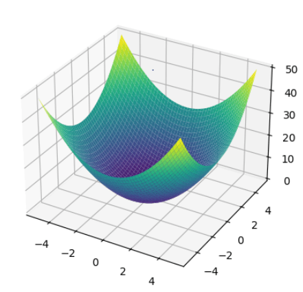
This function creates a surface. Our goal is to “minimize” the function, i.e. to find the lowest point on that surface. For a simple function like this we may be able to find it analytically. To do this, we would find the derivative of the function with respect to the parameters, set it equal to 0, and solve.

When training neural nets though, our function is often far too complicated to find the minimum analytically.

Instead, we start by picking any starting point on the surface, and computing the gradient of the function at that point. The gradient at that point is a vector that points in the direction of steepest ascent. If we move some small amount in the opposite direction of that gradient we will “descend” the surface of the function in careful steps. We can do this iteratively until the gradient gets close enough to 0.

This algorithm is called gradient descent. In many contexts in machine learning, the goal is to find the global minimum (for an example, read my series about SVMs). For training neural nets however, we give up on finding a global minimum and just try to get a very low value of the loss function.

Stochastic gradient descent is an optimization for the standard gradient descent algorithm based on one fact: the true gradient of the loss using all of the inputs is approximately the same as the gradient of the loss using a small random sample.

In this blog post we will be taking this idea to the extreme, and use only one randomly selected training example for each iteration of gradient descent.

Training Our Neural Net

Before we can actually implement stochastic gradient descent, we need a way to select random training examples.

This code ought to be pretty self-explanatory:

import random

def random_choice(l):
    return l[random.randint(0, len(l) - 1)]
    
def random_training_example():
    return random_choice(inputs)

Now, we can begin implementing SGD. In the section above I said that we descend the function in “small careful steps”. To be concrete about it, we select a learning rate: , a multiplier to the gradient that determines how large of a step we take relative to the size of the gradient. This is a hyperparameter; it is not learned during training.

eta = 0.0005

I’ve played around with learning rates and found that this works pretty well. If you were implementing your own neural net, a good method for choosing a learning rate is to start with a learning rate of 1, and then increase or decrease it by an order of magnitude depending on how training goes. For example, if you start at 1 and find that training is too slow, increase it to 10. If your step size is too large and your loss function starts increasing, move it down to 0.1. Once you have found a ballpark for the learning rate you can start to fine-tune it from there.

There are also methods for changing the learning rate during training. The gist is that you start with a larger learning rate, taking large steps when you are very far from a minimum then shrink the learning rate as training progresses. As you approach the minimum you need to make more careful steps so that you do not to overshoot the minimum. That is beyond the scope of this blog post, but I encourage you to look into it.

Our training loop is essentially this:

1. Pick a random training example (name and target letters).
2. Feed it through the forward pass.
3. Compute the loss.
4. Compute the gradients with backpropagation.
5. Move in the opposite direction of the gradient.
6. Repeat.

Here is the train() method in its entirety.

eta = 0.0005

def train(input, target):
    loss = 0
    
    hidden = rnn.init_hidden()
    os = np.zeros((input.shape[0], rnn.output_size))
    hs = np.zeros((input.shape[0], rnn.hidden_size)) 
    
    for i in range(input.shape[0]):
        output, hidden = rnn.forward(input[i], hidden)
        os[i] = output
        hs[i] = hidden

    for t, (y_hat, target_seq) in enumerate(zip(os, target)):
         target_index = target_seq.argmax().item()
         loss += -np.log(y_hat[target_seq.argmax().item()])

    dLdV, dLdW, dLdU, dLdc, dLdb = rnn.backward(input, target, os, hs)    

    rnn.V -= dLdV * eta
    rnn.W -= dLdW * eta
    rnn.U -= dLdU * eta
    rnn.c -= dLdc * eta
    rnn.b -= dLdb * eta

    return os, loss.item() / len(input)

This method performs one iteration of gradient descent. To fully train our network, we need to repeat this for some large number of iterations, with a new random training example each time.

n_iters = 100000
all_losses = []
total_loss = 0
plot_every = 500
print_every = 5000

for iter in range(1, n_iters + 1):
    
    output, l = train(*random_training_example(), False)
    total_loss += l

    if iter % print_every == 0:
        print(iter, iter / n_iters * 100, l)

    if iter % plot_every == 0:
        all_losses.append(total_loss / plot_every)
        total_loss = 0

As you can see we’re keeping track of the loss values as we train to monitor our progress. This is so that we can tell that our training is actually working.

Once training is complete, we can plot our losses to see the results:

import matplotlib.pyplot as plt

plt.figure()
plt.plot(all_losses)

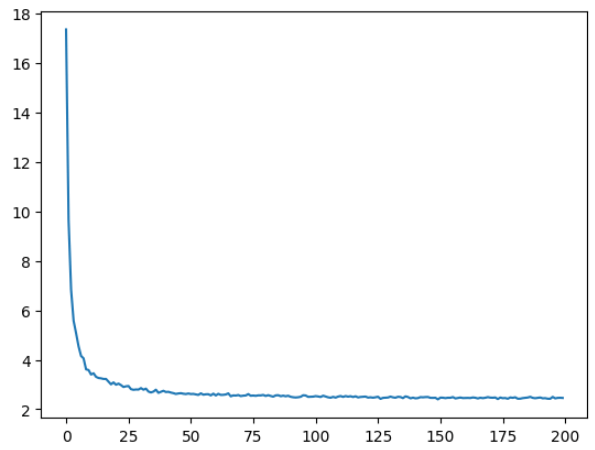
As you can see, we’ve successfully driven the value of our loss down. In the first few iterations our loss value dropped dramatically, and then plateaued between 2 and 4.

Sampling

Now that we’ve successfully trained our recurrent neural net we can finally generate some fake names!

The process of sampling from our network is pretty simple:

1. Pick a random starting letter.
2. Feed that letter through the net and get a new letter as output.
3. Repeat that iteratively until
   • Our “end of sequence” token is genrated
   • We reach some maximum length.

To make things a bit more interesting, we will be interpreting our output layer as a multinomial distribution and sampling from it randomly. If we simply chose the highest probability character every time, we’d get the same name for each starting letter.

There are more complicated sampling schemes, but this works well enough:

max_length = 20
num_samples = 5

# Sample from a category and starting letter
def sample(start_letter):
    input = name_tensor(start_letter)
    hidden = rnn.init_hidden()

    output_name = start_letter

    for i in range(max_length):
        output, hidden = rnn.forward(input[0], hidden)
        generated_char = index_to_char[np.random.multinomial(1, output).argmax()]
        if generated_char == '<E>':
            break
        else:
            letter = generated_char
            output_name += letter
        input = name_tensor(letter)

    return output_name

for i in range(num_samples):
    print(sample(random_choice(chars)))

Here’s some examples of names our recurrent neural net generated:

• masy
• romaon
• kymlieen
• halei
• elrsanth

You probably don’t know anyone with these names, and yet these are very “name like” sequences. Our recurrent neural net has successfully learned something fundamental about what makes a sequence of characters a name.

Conclusion

We have now successfully walked through a simple recurrent neural network implementation from scratch, and even used it to generate some fake names for us.

I hope that you’ve enjoyed this series so far. In the next blog post I will be discussing next steps, some of the fundamental problems with recurrent neural nets, and how we can address them.

Thank you for reading!