
I think it is useful to learn backpropagation outside the context of neural nets first until you gain the intuition. Once you have gained the intuition, the equations involved in backpropagating error through a neural net are much easier to understand.
Backpropagation is nothing more than the chain rule from calculus.
Chain Rule
For any nested function: 


Consider the function:

This function can really be thought of as two nested functions:


So, according to the chain rule, to find 

and multiply it by the derivative of the outer function if the inner function were just a variable:

Backpropagation with a simple function
Let’s define a function, 

Let’s define some intermediate variables that are the result of operations on the variables we just defined:


With these new intermediate variables we can rewrite


We can now assign values to our variables and evaluate


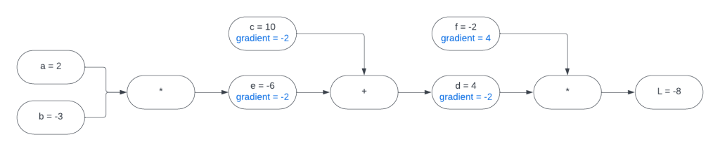
Here is a visual representation of our expression graph:

As you can see by looking at this graph, 

To find the derivative of


Let’s fill those gradients in on our graph:

Now we want to find the gradients for 

Taking a look at our expression graph we can see two important facts:


In other words,
We computed the derivative of the “outer function” in the previous step.

We only need to calculate the derivative of the “inner function” and multiply it by 


The gradient for 

First we can find the gradient for


Filling in those gradients on our expression graph:
Let’s finish this off and find the gradients for


These are nested functions and we can find their gradients using the chain rule. The “outer function” this time is 


Here’s the final expression graph:

We just found all of the gradients in this expression graph using backpropagation. In case it was not obvious, I called this function
The Four Fundamental Equations of Backpropagation
To make things easy for the initial explanation I will pretend that our neural net has only 3 neurons: 1 input, 1 hidden layer neuron, and 1 output neuron.
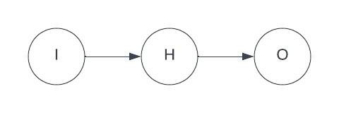
I think it is easier to understand how the equations are derived in the context of a simple net like this. Once you understand that, the only difference between it and a more complicated net is using vectors and matrices to group things together. The equations are essentially the same.
The First Fundamental Equation of Backpropagation
The real implementation of backpropagation I will show works on a layer by layer basis, but this is just for efficiency. In the toy example above we broke up each operation into its simplest possible expression. In either case, the gradients you get will be the same. It does not matter how fine-grained you choose to break your nested functions down.
For each layer we will be calculating a value called the error, denoted by the Greek symbol 

First, we must calculate the error of the output layer.
The loss function is a function of the output. Let’s call the output, 

The output is a function of the weighted sum. It is the weighted sum after activation:

I hope this is starting to look familiar at this point. This is another nested function:

We can apply the chain rule to find the gradient of 

In the case of the quadratic loss function we are using, the derivative of the loss function with respect to the output is:

Where 
To find the derivative of the “inner function” we really just pass the weighted sum into the derivative of the activation function:

Putting these two together yields our first fundamental equation:

The Second Fundamental Equation of Backpropagation
Now we need some way of using this error to find the error in the previous layers.
The weighted sum of any layer in the network is a function of the weighted sum of the layer before it. For any layer, the weighted sum of the next layer is defined in terms of the weighted sum of the current layer with this equation:

This is another application of the chain rule.

For our hidden layer, we already know the derivative of the loss with respect to the weighted sum of the output layer. We calculated that in the first equation. It’s 

Putting these two together gives us:

This is the second fundamental equation.
The 
The Third Fundamental Equation of Backpropagation
Now that we have the error for all of our layers we can use it to find the gradients of the weights and biases.
How do we find the gradient of the biases using the error? The error is the gradient of the bias. This is really no surprise because the weighted sum is a function of the bias:

This is another application of the chain rule:

The derivative of the “outer function” is

Since

Putting it together:

The Fourth Fundamental Equation of Backpropagation
All that’s left is to find the gradient of the weights using the error. Once again we apply the chain rule:

All that’s left is to find the local derivative: 


Putting these two together gives us:

Conclusion
That’s how we use backpropagation to find the gradients of the weights and biases in the network.
The only three changes we need to make to the equations to accommodate a neural net of arbitrary size are:
- All of the
s would be matrices.
- For the second fundamental equation, the
in the equation is actually the transpose of the weight matrix of the next layer. This would be more accurately written as
. In our one-neuron-per-layer example it didn’t matter. I think the relationship between this equation and the chain rule is made more obvious if
- The multiplication of vectors in these equations represents the Hadamard product. The Hadamard product is just the result of entry-wise multiplication of two vectors.
In the next blog post I will show how to actually implement the four fundamental equations of backpropagation in code.

Leave a reply to The Cross-Entropy Loss Function – Robert Vagene's Blog Cancel reply